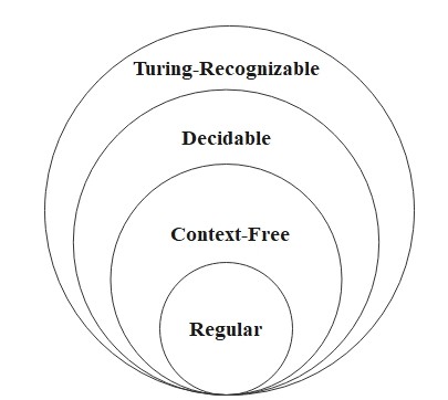
Turing Machines

Example:

Consider the language \[ L_1 = \{0^{2^n} \mid n \geq 0\}, \] which consists of all strings of \(0\)s whose length is a power of 2.

The following Turing machine \(M_1\) decides \(L_1\):

\(M_1 = \) "On input string \(w\):

1. Read left to right across the tape, crossing out every other \(0\).
2. If in Stage 1, the tape contained a single \(0\), accept.
3. If in Stage 1, the tape contained no \(0\), or more than a single \(0\) with the number of \(0\)s odd, reject.
4. Return the head to the left-hand end of the tape.
5. Go back to Stage 1."

In the state diagram below, Stage 1's "crossing out every other \(0\)" is realized in two steps. The machine first replaces the leftmost \(0\) with a blank \(\sqcup\), which serves as the left-end marker that the head returns to in Stage 4. It then replaces every other subsequent \(0\) with \(\text{x}\). The trace that follows illustrates exactly this behavior.

Here \(Q = \{q_1, q_2, q_3, q_4, q_5, q_{\mathrm{accept}}, q_{\mathrm{reject}}\}\), \(\Sigma = \{0\}\), and \(\Gamma = \{0, \text{x}, \sqcup\}\). The state diagram of \(M_1\) is as follows:

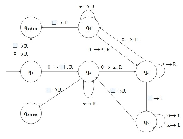
For example, if the input is \(0000\), the sequence of configurations is as follows: \[ \begin{align*} &q_1 0 0 0 0 \vdash \sqcup q_2 0 0 0 \vdash \sqcup \text{x} q_3 0 0 \vdash \sqcup \text{x} 0 q_4 0 \\\\ &\vdash \sqcup \text{x} 0 \text{x} q_3 \sqcup \vdash \sqcup \text{x} 0 q_5 \text{x} \sqcup \vdash \sqcup \text{x} q_5 0 \text{x} \sqcup \\\\ &\vdash \sqcup q_5 \text{x} 0 \text{x} \sqcup \vdash q_5 \sqcup \text{x} 0 \text{x} \sqcup \vdash \sqcup q_2 \text{x} 0 \text{x} \sqcup \\\\ &\vdash \sqcup \text{x} q_2 0 \text{x} \sqcup \vdash \sqcup \text{x} \text{x} q_3 \text{x} \sqcup \vdash \sqcup \text{x} \text{x} \text{x} q_3 \sqcup \\\\ &\vdash \sqcup \text{x} \text{x} q_5 \text{x} \sqcup \vdash \sqcup \text{x} q_5 \text{x} \text{x} \sqcup \vdash \sqcup q_5 \text{x} \text{x} \text{x} \sqcup \\\\ &\vdash q_5 \sqcup \text{x} \text{x} \text{x} \sqcup \vdash \sqcup q_2 \text{x} \text{x} \text{x} \sqcup \vdash \sqcup \text{x} q_2 \text{x} \text{x} \sqcup \\\\ &\vdash \sqcup \text{x} \text{x} q_2 \text{x} \sqcup \vdash \sqcup \text{x} \text{x} \text{x} q_2 \sqcup \\\\ &\vdash \sqcup \text{x} \text{x} \text{x} \sqcup q_{\mathrm{accept}}. \end{align*} \]

Proof sketch.

Given a \(k\)-tape Turing machine \(M\), we construct a single-tape machine \(T\) that simulates \(M\). The single tape of \(T\) represents the contents of all \(k\) tapes of \(M\) by storing them consecutively, separated by a fresh delimiter symbol \(\#\): \[ \# \, \text{tape}_1 \, \# \, \text{tape}_2 \, \# \, \cdots \, \# \, \text{tape}_k \, \#. \] To track each head's position, \(T\) marks the cell where \(M\)'s head currently sits on each tape with a "dotted" version of that symbol (a new symbol added to the tape alphabet). For instance, if \(M\)'s tape \(i\) contains \(010\) with the head on the middle \(1\), \(T\) records \(\#0\dot{1}0\#\).

On input \(w\), \(T\) first formats its tape into this representation (with \(w\) on tape 1 and the remaining tapes blank). To simulate one step of \(M\), \(T\) scans across its tape from the leftmost \(\#\) to the \((k+1)\)-st \(\#\) to read the symbols under all virtual heads, then makes a second pass to update the contents and head positions according to \(M\)'s transition function.

If a virtual head moves rightward onto a delimiter \(\#\), \(T\) shifts that delimiter, together with all tape contents to its right, one cell further right, and writes a dotted blank in the vacated cell. The virtual head now occupies this fresh blank cell. If a virtual head would move left from the first cell of its tape, \(T\) leaves it in place, following for each tape of \(M\) the convention that a left move from the leftmost cell does not move the head. The machine \(T\) accepts (or rejects) precisely when \(M\) does. Hence \(T\) recognizes the same language as \(M\).

Proof sketch.

We sketch each claim in turn.

Claim 1 (every CFL is decidable). Given a CFL \(L\) generated by a context-free grammar \(G\), the membership question "is \(w \in L\)?" can be decided by the Cocke-Younger-Kasami (CYK) algorithm. We assume that \(G\) has been converted into Chomsky Normal Form beforehand. This conversion is a fixed transformation of the grammar, not part of processing the input. The algorithm uses dynamic programming to build up the set of variables that can derive each substring of \(w\), and it accepts if and only if the start variable derives \(w\) itself. The procedure performs \(O(|w|^3)\) table operations and in particular halts on every input, so the Turing machine implementing it decides \(L\).

Claim 2 (some Turing-recognizable languages are undecidable). The canonical example is the acceptance problem \[ A_{\mathrm{TM}} = \{ \langle M, w \rangle \mid M \text{ is a Turing machine that accepts } w \}. \] The language \(A_{\mathrm{TM}}\) is Turing-recognizable. A universal Turing machine takes \(\langle M, w \rangle\) as input, simulates \(M\) on \(w\), and accepts whenever \(M\) accepts. However, \(A_{\mathrm{TM}}\) is undecidable. The proof, a modern form of Turing's diagonal argument, is analogous to the one we develop in the next section. Suppose \(H\) were a decider for \(A_{\mathrm{TM}}\). Let \(D\) be the machine that, on input \(\langle M \rangle\), runs \(H\) on \(\langle M, \langle M \rangle \rangle\) and outputs the opposite answer, rejecting if \(H\) accepts and accepting if \(H\) rejects. Since \(H\) always halts, so does \(D\), and \(D\) accepts \(\langle M \rangle\) exactly when \(M\) does not accept \(\langle M \rangle\). Running \(D\) on its own description \(\langle D \rangle\) then gives that \(D\) accepts \(\langle D \rangle\) if and only if \(D\) does not accept \(\langle D \rangle\), a contradiction.

Claim 3 (decidable if and only if Turing-recognizable and co-Turing-recognizable). (\(\Rightarrow\)) If \(L\) is decidable, a decider \(M\) for \(L\) recognizes \(L\), so \(L\) is Turing-recognizable. Swapping \(q_{\mathrm{accept}}\) and \(q_{\mathrm{reject}}\) in \(M\) yields a decider, hence a recognizer, for \(L^c\). (\(\Leftarrow\)) Suppose \(M_1\) recognizes \(L\) and \(M_2\) recognizes \(L^c\). We build a new Turing machine \(M\) that, on input \(w\), simulates \(M_1\) and \(M_2\) in parallel step by step (advancing each machine by one step in alternation, on a shared input). Since every \(w\) lies in exactly one of \(L\) or \(L^c\), exactly one of \(M_1, M_2\) eventually accepts. The machine \(M\) halts and accepts (resp. rejects) when \(M_1\) (resp. \(M_2\)) accepts. Thus \(M\) decides \(L\).

Proof.

Suppose for contradiction that \(f: X \to \mathcal{P}(X)\) is a bijection. Define the set \[ D = \{ x \in X \mid x \notin f(x) \} \in \mathcal{P}(X). \] Since \(f\) is surjective, there exists \(d \in X\) with \(f(d) = D\). Now ask: is \(d \in D\)?

• If \(d \in D\), then by definition of \(D\) we have \(d \notin f(d) = D\), a contradiction.
• If \(d \notin D\), then by definition of \(D\) we have \(d \in f(d) = D\), a contradiction.

Either case is contradictory, so no such bijection \(f\) exists. The argument used only the surjectivity of \(f\), so in fact no map \(X \to \mathcal{P}(X)\) is surjective. Taking \(X = \mathbb{N}\) shows that \(\mathcal{P}(\mathbb{N})\) is uncountable. Indeed, by definition a set is countable if and only if it is in bijection with \(\mathbb{N}\) or with a subset of \(\mathbb{N}\). If \(g: S \to \mathcal{P}(\mathbb{N})\) were a bijection with \(S \subseteq \mathbb{N}\), then \(S\) would be nonempty, because \(\mathcal{P}(\mathbb{N})\) is nonempty. Fixing \(s_0 \in S\) and sending every element of \(\mathbb{N} \setminus S\) to \(g(s_0)\) would then extend \(g\) to a surjection \(\mathbb{N} \to \mathcal{P}(\mathbb{N})\), which is impossible.

Proof.

Fix a nonempty finite alphabet \(\Sigma\). First, we show that, up to renaming, the Turing machines with input alphabet \(\Sigma\) form a countable set. Renaming the states or the tape symbols outside \(\Sigma \cup \{\sqcup\}\) does not change the language a machine recognizes, so we may assume that the states are drawn from a fixed list \(q_1, q_2, \ldots\) and those tape symbols from a fixed list \(\gamma_1, \gamma_2, \ldots\), and we count only such machines. Each such machine \(M\) can then be encoded as a finite string \(\langle M \rangle\) over some fixed finite alphabet \(\Delta\). For instance, we can serialize its 7-tuple specification with appropriate delimiters so that distinct machines produce distinct strings.

The set \(\Delta^*\) of all strings over \(\Delta\) can be written as \[ \Delta^* = \bigcup_{n \geq 0} \Delta^n, \] where \(\Delta^n\) is the set of strings of length \(n\). Each \(\Delta^n\) is finite, so listing the strings of \(\Delta^0\), then those of \(\Delta^1\), and so on, gives a list in which every string of \(\Delta^*\) appears exactly once at a finite position. Hence \(\Delta^*\) is countable. The encoding \(M \mapsto \langle M \rangle\) is injective, so the set of machines we count is in bijection with a subset of \(\Delta^*\), and hence is also countable.

Next, we show that the set of all languages over \(\Sigma\) is uncountable. A language over \(\Sigma\) is, by definition, any subset of \(\Sigma^*\), so the set of all languages is exactly \(\mathcal{P}(\Sigma^*)\). The same listing, applied to \(\Sigma\), enumerates every string of \(\Sigma^*\) exactly once. Since \(\Sigma\) is nonempty, the list is infinite, so it puts \(\Sigma^*\) in bijection with \(\mathbb{N}\). Transporting Cantor's theorem along this bijection, we conclude that \(\mathcal{P}(\Sigma^*)\) is uncountable.

Every Turing-recognizable language over \(\Sigma\) is recognized by one of the machines we count. Indeed, a recognizer whose input alphabet differs from \(\Sigma\) can be converted into one with input alphabet exactly \(\Sigma\): after any auxiliary tape symbol of the original machine that lies in \(\Sigma\) is renamed to a fresh symbol outside \(\Sigma\), the original machine's input symbols outside \(\Sigma\) become auxiliary tape symbols, and a preliminary scan rejects any input containing a symbol of \(\Sigma\) outside the original input alphabet. Since each machine we count recognizes exactly one language over \(\Sigma\), the recognizable languages over \(\Sigma\) are the image of a countable set and therefore form a countable set, while the set of all languages over \(\Sigma\) is uncountable. Hence some language over \(\Sigma\) cannot be recognized by any Turing machine.