Introduction
Automata theory is a foundational area of theoretical computer science and discrete mathematics that studies abstract
machines and computational problems. It provides a rigorous framework for understanding formal languages, state-based
computation, and algorithmic processes. For instance, automata theory is essential in compiler design, natural language processing,
software verification, and the study of complexity classes in the theory of computation. By exploring automata theory, we
will develop a deeper understanding of computation, logic, and the mathematical principles governing algorithmic processes.
In this page, we introduce the simplest computational model — the finite automaton -
and the class of languages it recognizes: regular languages. We then study the regular
operations (union, concatenation, and Kleene star), the equivalence between deterministic and nondeterministic
machines, and the connection to regular expressions.
Finite Automata & Regular Languages
Real computers are enormously complex, so to study the fundamental principles of computation, we introduce
simplified computational models that isolate specific features. The simplest such model
is the finite automaton (also called a finite state machine).
Definition: Finite Automaton (DFA)
A finite automaton is a 5-tuple \((Q, \Sigma, \delta, q_0, F)\) where
- \(Q\) is a finite set called the states,
- \(\Sigma\) is a finite set called the alphabet,
- \(\delta: Q \times \Sigma \to Q\) is the transition function,
- \(q_0 \in Q\) is the start state,
- \(F \subseteq Q\) is the set of accept states.
Given an input string \(w = w_1 w_2 \cdots w_n\) over \(\Sigma\), the machine starts in state \(q_0\) and
reads \(w\) one symbol at a time, transitioning according to \(\delta\). After reading the final symbol,
if the resulting state lies in \(F\) we say \(M\) accepts \(w\); otherwise \(M\)
rejects \(w\). Let \(A\) be the set of all strings that \(M\) accepts. We say \(A\) is the
language of \(M\) and write:
\[
L(M) = A
\]
We also say that \(M\) recognizes \(A\). Moreover, a language is called a
regular language if some finite automaton recognizes it.
Definition: Computation and Acceptance
Let \(M = (Q, \Sigma, \delta, q_0, F)\) be a finite automaton and let \(w = w_1 w_2 \cdots w_n\) be a
string over \(\Sigma\) (where each \(w_i \in \Sigma\), and the case \(n = 0\) corresponds to the empty
string \(\epsilon\)). A computation of \(M\) on \(w\) is a sequence of states
\(r_0, r_1, \ldots, r_n \in Q\) satisfying:
- \(r_0 = q_0\),
- \(r_{i+1} = \delta(r_i, w_{i+1})\) for each \(i = 0, 1, \ldots, n-1\).
We say that \(M\) accepts \(w\) if \(r_n \in F\), and rejects \(w\)
otherwise. The language recognized by \(M\) is then defined formally as
\[
L(M) = \{\, w \in \Sigma^* \mid M \text{ accepts } w \,\}.
\]
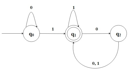
Consider the following finite automaton.
First, this directed multigraph is called the state diagram of the finite automaton.
It has three states, \(Q = \{q_0, q_1, q_2\}\), where \(q_0\) is the start state, and \(F = \{q_1\}\) is the
accept state which is denoted by a double circle. The arrows are transitions \(\delta\) from one state to another state.
This automaton processes an input string over the alphabet (in this case, \(\Sigma = \{0, 1\}\)) and returns either
"accept" or "reject" as output.
For example, if the input string is 1101101, this automaton processes the string as follows:
Start reading
Read 1, move from \(q_0\) to \(q_1\)
Read 1, stay in \(q_1\)
Read 0, move to \(q_2\)
Read 1, move to \(q_1\)
Read 1, stay in \(q_1\)
Read 0, move to \(q_2\)
Read 1, move to \(q_1\)
End reading
Return "accept."
This automaton recognizes strings that end with a 1 followed by an even number of 0s. For example, 10100 is
accepted because it ends with 1 followed by two 0s, but 1011000 is rejected because it ends with three 0s after
the last 1. Note that a string ending in 1 (with zero trailing 0s) is also accepted, since zero is even.
Regular Operations
We now define three fundamental operations on languages. A key result is that regular languages are
closed under all three - applying any of these operations to regular languages always yields
another regular language.
Definition: Regular Operations
Let \(A\) and \(B\) be languages over an alphabet \(\Sigma\).
- Union:
\(A \cup B = \{x \mid x \in A \text{ or } x \in B\}\)
- Concatenation:
\(A \circ B = \{xy \mid x \in A \text{ and } y \in B\}\)
Note: \(\emptyset \circ A = \emptyset\), and \(\{\epsilon\} \circ A = A\).
Also, \(A \circ A = A^2\), and we define \(A^0 = \{\epsilon\}\).
- Kleene Star:
\(A^* = \{x_1 x_2 \cdots x_k \mid k \geq 0 \text{ and each } x_i \in A\}\)
Equivalently, \(A^* = A^0 \cup A^1 \cup A^2 \cup \cdots\).
Note: The empty string \(\epsilon\) is always in \(A^*\) (the case \(k = 0\)).
In particular, \(\emptyset^* = \{\epsilon\}\)
since \(\emptyset^* = \emptyset^0 \cup \emptyset^1 \cup \emptyset^2 \cup \cdots\).
For example, Let \(\Sigma = \{a, \, b, \, c, \, \cdots, \, x, \, y, \, z\}\).
If \(A = \{black, \, white\}\) and \(B = \{dog, \, cat\}\), then
\[
\begin{align*}
&A \cup B = \{black, \, white, \, dog, \, cat \} \\\\
&A \circ B = \{blackdog, \, blackcat, \, whitedog, \, whitecat\} \\\\
&A^* = \{\epsilon, \, black, \, white, \, blackblack, \, blackwhite, \, whiteblack, \, whitewhite, \, blackblackblack, \, blackblackwhite, \, \cdots\}
\end{align*}
\]
Theorem 1: Closure of Regular Languages
The class of regular languages is closed under the regular operations. That is,
if \(A\) and \(B\) are regular languages, then \(A \cup B\), \(A \circ B\),
\(A^*\), and \(B^*\) are also regular.
Proof: Closure under union
Suppose we have two finite automata
\[
M_1 = (Q_1, \Sigma, \delta_1, q_{0_1}, F_1)
\]
and
\[
M_2 = (Q_2, \Sigma, \delta_2, q_{0_2}, F_2).
\]
These can recognize regular languages \(A_1\) and \(A_2\) respectively.
Here, we can construct \(M_3\) to recognize \(A_1 \cup A_2\) as follows:
\[
M_3 = (Q_3, \Sigma, \delta_3, q_{0_3}, F_3)
\]
where
\[
Q_3 = Q_1 \times Q_2 = \{(q_1, q_2)\, | \, q_1 \in Q_1 \text{ and } q_2 \in Q_2\}
\]
\[
\delta_3((q_1, q_2), a) = (\delta_1(q_1, a), \delta_2(q_2, a)) \quad \forall a \in \Sigma
\]
\[
q_{0_3} = (q_{0_1}, q_{0_2})
\]
\[
F_3 = \{(q_1, q_2) \,| \, q_1 \in F_1 \text{ or } q_2 \in F_2 \}
\]
which is the same as \((F_1 \times Q_2) \cup (Q_1 \times F_2)\).
Verification.
The key claim is the following: for any input string \(w\), after \(M_3\)
reads \(w\), its state is exactly \((r_1, r_2)\), where \(r_i\) is the state \(M_i\) reaches after reading
\(w\). This follows by a straightforward induction on \(|w|\), the crucial point being that \(\delta_3\)
acts component-wise — at every step, the first component is updated by \(\delta_1\) and the
second by \(\delta_2\) independently. Once this claim is established, the acceptance condition unfolds as
\[
M_3 \text{ accepts } w \iff (r_1, r_2) \in F_3 \iff r_1 \in F_1 \text{ or } r_2 \in F_2 \iff M_1 \text{ accepts } w \text{ or } M_2 \text{ accepts } w.
\]
Therefore \(L(M_3) = A_1 \cup A_2\), proving that \(A_1 \cup A_2\) is regular.
Note: The same product construction with \(F_3 = F_1 \times F_2\) (instead of the union of slices) recognizes
\(A_1 \cap A_2\), since now \(M_3\) accepts only when both \(M_1\) and \(M_2\) accept. This shows
that the class of regular languages is also closed under intersection.
Closure under concatenation and Kleene star.
The product construction we just used for union
does not adapt cleanly to concatenation or Kleene star. The reason is that a DFA reading \(w\) must commit,
at every position, to a single next state — but to recognize \(A_1 \circ A_2\), the machine would need to
decide where the prefix from \(A_1\) ends and the suffix from \(A_2\) begins, and this split point is not
visible from the input alone. Similarly for \(A^*\), the machine would need to decide how many times to
re-enter \(A\) and where each repetition begins.
The natural way to handle this is to allow the machine to "guess" — that is, to use a
nondeterministic finite automaton (NFA), introduced in the next section. Once NFAs are
available, the constructions become straightforward: for concatenation, glue the accept states of an NFA
for \(A_1\) to the start state of an NFA for \(A_2\) via \(\epsilon\)-transitions; for Kleene star, add a
new start state that loops back from each old accept state. The explicit constructions appear in the proof
of Theorem 3
(cases 5 and 6 of Part 1). Combined with the
NFA-DFA equivalence,
these show that if \(A_1, A_2\) are regular — that is, recognized by some DFAs, which can themselves be
viewed as NFAs — then \(A_1 \circ A_2\) and \(A_1^*\) are recognized by NFAs (by the constructions just
sketched), and therefore by DFAs (by the equivalence). Hence \(A_1 \circ A_2\) and \(A_1^*\) are regular,
completing the closure result.
Deterministic & Nondeterministic Machine
So far, we have considered deterministic computation: at each step, the current state and input
symbol uniquely determine the next state. However, what if a computation is allowed multiple choices for the
next state? Such a computation is called nondeterministic. Every deterministic finite automaton
(DFA) is trivially a nondeterministic finite automaton (NFA), since determinism
is a special case of nondeterminism. Formally, given a DFA with transition function
\(\delta_D: Q \times \Sigma \to Q\), we view it as an NFA by setting
\(\delta_N(q, a) = \{\delta_D(q, a)\}\) for each \(a \in \Sigma\) and \(\delta_N(q, \epsilon) = \emptyset\).
Definition: Nondeterministic Finite Automaton (NFA)
A nondeterministic finite automaton is a 5-tuple \((Q, \Sigma, \delta, q_0, F)\) where
- \(Q\) is a finite set of states,
- \(\Sigma\) is a finite alphabet,
- \(\delta: Q \times \Sigma_{\epsilon} \to \mathcal{P}(Q)\) is the transition function,
- \(q_0 \in Q\) is the start state,
- \(F \subseteq Q\) is the set of accept states,
where \(\Sigma_{\epsilon} = \Sigma \cup \{\epsilon\}\) and \(\mathcal{P}(Q)\) is the power set of \(Q\).
The transition \(\delta(q, \epsilon)\) defines an \(\epsilon\)-transition: the NFA may move
from state \(q\) to any state in \(\delta(q, \epsilon)\) without consuming any input symbol. This
is one of the key features that distinguishes NFAs from DFAs and will play a central role when we build
NFAs from regular expressions in the next section.
Note: The power set of a set is the set of all possible subsets of that set, including the empty set and the set itself. For example,
if \(Q = \{a, b, c\}\), then \(\mathcal{P}(Q) = \{\emptyset, \{a\}, \{b\}, \{c\}, \{a, b\}, \{a, c\}, \{b, c\}, \{a, b, c\}\} \). So, if
a set has \(n\) elements, its power set has \(2^n\) elements.
At each state, the NFA can split itself into multiple branches and keeps following all the possible branches in parallel.
In other words, the NFA can have multiple active states at once, while the DFA always has a single active state.
If at least one of these branches reaches an accept state, then the whole computation accepts.
Note: The NFA sounds like parallel computation, but in "actual" parallel computation, multiple processors or threads execute
tasks concurrently, often with considerations for synchronization, communication, and resource sharing. NFAs don't model
these practical concerns.
Theorem 2: NFA-DFA Equivalence
Every NFA has an equivalent DFA. That is, for every NFA \(N\), there exists a DFA \(D\)
such that \(L(N) = L(D)\).
Proof Sketch (Subset Construction)
Let \(N = (Q, \Sigma, \delta, q_0, F)\) be an NFA. The key idea is that since \(N\) can be in several
states simultaneously, a single state of the equivalent DFA should encode which subset of \(Q\)
the NFA is currently in. We first treat the case without \(\epsilon\)-transitions; the general case
is handled by a small modification described at the end.
Construct \(D = (Q', \Sigma, \delta', q_0', F')\) as follows:
- \(Q' = \mathcal{P}(Q)\) — each DFA state is a subset of NFA states.
- \(\delta'(R, a) = \displaystyle\bigcup_{r \in R} \delta(r, a)\) — from a subset \(R\), the new subset is the union of all states reachable from any \(r \in R\) on input \(a\).
- \(q_0' = \{q_0\}\) — the DFA starts in the singleton subset containing the NFA's start state.
- \(F' = \{R \subseteq Q \mid R \cap F \neq \emptyset\}\) — a subset is accepting if it contains at least one NFA accept state.
Correctness. By induction on the length of the input, one shows that after reading
\(w = w_1 w_2 \cdots w_n\), the DFA \(D\) is in the state \(R_n \subseteq Q\) consisting of exactly
those NFA states that \(N\) can reach after reading \(w\). Therefore \(D\) accepts \(w\) if and only if
some such reachable state lies in \(F\), which is precisely the condition for \(N\) to accept \(w\).
Hence \(L(D) = L(N)\).
Handling \(\epsilon\)-transitions. For each \(R \subseteq Q\), define the
\(\epsilon\)-closure \(E(R)\) as the set of all states reachable from \(R\) by following
zero or more \(\epsilon\)-transitions. Modify the construction by setting
\(\delta'(R, a) = E\bigl(\bigcup_{r \in R} \delta(r, a)\bigr)\) and
\(q_0' = E(\{q_0\})\). The same inductive argument then carries through.
Importantly, this theorem says that NFAs and DFAs recognize the same class of languages - the
regular languages. However, an NFA is often much smaller and easier to design than its equivalent DFA. The
conversion (known as the power set construction or subset construction) can
produce a DFA with up to \(2^{|Q|}\) states, so the two models are not equivalent in terms of succinctness.
We now introduce a third way to describe regular languages - through algebraic expressions rather than machines.
Regular Expressions
Definition: Regular Expression
\(R\) is a regular expression over the alphabet \(\Sigma\) if \(R\) is one of the following:
- \(a\) for some \(a \in \Sigma\) (the language \(\{a\}\)),
- \(\epsilon\) (the language \(\{\epsilon\}\) containing only the empty string),
- \(\emptyset\) (the empty language, containing no strings),
- \((R_1 \cup R_2)\), where \(R_1\) and \(R_2\) are regular expressions,
- \((R_1 \circ R_2)\), where \(R_1\) and \(R_2\) are regular expressions,
- \((R_1^*)\), where \(R_1\) is a regular expression.
This is an inductive definition: cases 4-6 build larger expressions from smaller ones.
A language that can be described by a regular expression is precisely a language recognizable by a
finite automaton — this is the reason such languages are called regular.
To distinguish a regular expression \(R\) from the language it describes, we write \(L(R)\) for
the language of \(R\).
Theorem 3: Equivalence of Regular Expressions and Finite Automata
A language is regular if and only if some regular expression describes it. That is:
- If a language is described by a regular expression, then it is regular.
- If a language is regular, then it is described by a regular expression.
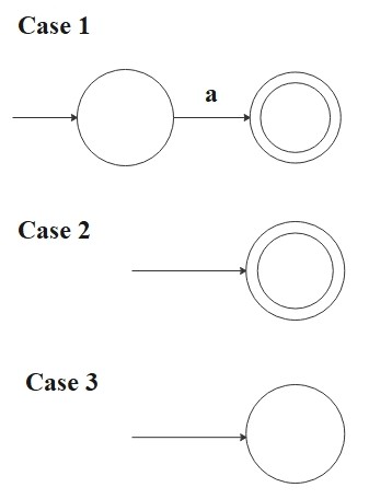
Proof: Part 1
The proof is by structural induction on the regular expression \(R\). The base cases
(1, 2, 3) handle the atomic regexes built without combination; the inductive cases (4, 5, 6) build an
NFA for \(R\) from NFAs for the smaller subexpressions \(R_1, R_2\). For each case, we exhibit an NFA
\(M\) recognizing \(L(R)\), which establishes regularity (since any language recognized by an NFA is
regular by Theorem 2).
- \(R = a\) for some \(a \in \Sigma\):
Then
\[
L(R) = \{a\}
\]
and the following NFA recognizes \(L(R)\):
\[
M = (\{q_0 , q_1\}, \Sigma, \delta, q_0, \{q_1\})
\]
where \(\delta(q_0, a) = \{q_1\}\) and \(\delta(r, b) = \emptyset\) for \(r \neq q_0\) or \(b \neq a\).
- \(R =\epsilon\):
Then
\[
L(R) = \{\epsilon\}
\]
and the following NFA recognizes \(L(R)\):
\[
M = (\{q_0\}, \Sigma, \delta, q_0, \{q_0\})
\]
where \(\delta(r, b) = \emptyset\) for any \(r\) and \(b\).
- \(R = \emptyset\):
Then
\[
L(R) = \emptyset
\]
and the following NFA recognizes \(L(R)\):
\[
M = (\{q\}, \Sigma, \delta, q, \emptyset)
\]
where \(\delta(r, b) = \emptyset\) for any \(r\) and \(b\).
For cases 4, 5, and 6, let \(M_1 = (Q_1, \Sigma, \delta_1, q_{0_1}, F_1)\) be an NFA that recognizes \(L(R_1)\) and
\(M_2 = (Q_2, \Sigma, \delta_2, q_{0_2}, F_2)\) be an NFA that recognizes \(L(R_2)\). We assume that the state sets
\(Q_1\) and \(Q_2\) are disjoint.
- \(R = (R_1 \cup R_2)\):
Then
\[
L(R) = L(R_1) \cup L(R_2)
\]
and the following NFA recognizes \(L(R)\):
\[
M = ( Q_1 \cup Q_2 \cup \{q_0\}, \Sigma, \delta, q_0, F_1 \cup F_2)
\]
where for any \(q \in Q\) and any \(a \in \Sigma_{\epsilon}\),
\[
\delta(q, a) = \begin{cases}
\delta_1(q, a) &\text{if \(q \in Q_1\)}, \\
\delta_2(q, a) &\text{if \(q \in Q_2\)}, \\
\{q_{0_1}, q_{0_2}\} &\text{if \(q = q_0\) and \(a = \epsilon\)}, \\
\emptyset &\text{if \(q = q_0\) and \(a \neq \epsilon\)}. \\
\end{cases}
\]
Verification.
On input \(w\), \(M\) starts at \(q_0\) and immediately \(\epsilon\)-branches
into both \(q_{0_1}\) and \(q_{0_2}\), after which the two branches process \(w\) as \(M_1\) and
\(M_2\) independently. Since the accept set is \(F_1 \cup F_2\), the machine \(M\) accepts iff at
least one of \(M_1, M_2\) accepts \(w\), i.e., iff \(w \in L(R_1) \cup L(R_2)\).

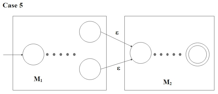
- \(R = (R_1 \circ R_2)\):
Then
\[
L(R) = L(R_1) \circ L(R_2)
\]
and the following NFA recognizes \(L(R)\):
\[
M = ( Q_1 \cup Q_2 , \Sigma, \delta, q_{0_1}, F_2)
\]
where for any \(q \in Q\) and any \(a \in \Sigma_{\epsilon}\),
\[
\delta(q, a) = \begin{cases}
\delta_1(q, a) &\text{if \(q \in Q_1\) and \(q \not\in F_1\) }, \\
\delta_1(q, a) &\text{if \(q \in F_1\) and \(a \neq \epsilon\) }, \\
\delta_1(q, a) \cup \{q_{0_2}\} &\text{if \(q \in F_1\) and \(a = \epsilon\) } \\
\delta_2(q, a) &\text{if \(q \in Q_2\) }. \\
\end{cases}
\]
Verification.
On input \(w\), \(M\) starts at \(q_{0_1}\) and processes \(w\) as \(M_1\).
Whenever computation enters an \(F_1\) state, an \(\epsilon\)-transition to \(q_{0_2}\) becomes
available — the NFA may nondeterministically take this transition or continue inside \(M_1\).
Once it jumps, the rest of \(w\) is processed as \(M_2\). Since the accept set is \(F_2\) only,
\(M\) accepts iff \(w\) splits as \(w = uv\) with \(u \in L(R_1)\) and \(v \in L(R_2)\), i.e.,
iff \(w \in L(R_1) \circ L(R_2)\).
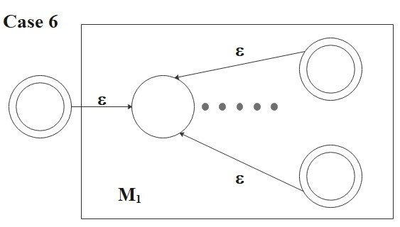
- \(R = (R_1^*) \):
Then
\[
L(R) = L(R_1)^*
\]
and the following NFA recognizes \(L(R)\):
\[
M = ( Q_1 \cup \{q_0\}, \Sigma, \delta, q_0, \{q_0\} \cup F_1)
\]
where for any \(q \in Q\) and any \(a \in \Sigma_{\epsilon}\),
\[
\delta(q, a) = \begin{cases}
\delta_1(q, a) &\text{if \(q \in Q_1\) and \(q \not\in F_1\) } \\
\delta_1(q, a) &\text{if \(q \in F_1\) and \(a \neq \epsilon\) }, \\
\delta_1(q, a) \cup \{q_{0_1}\} &\text{if \(q \in F_1\) and \(a = \epsilon\) }, \\
\{q_{0_1}\} &\text{if \(q = q_0\) and \(a = \epsilon\) }, \\
\emptyset &\text{if \(q=q_0\) and \(a \neq \epsilon\)}. \\
\end{cases}
\]
Verification. The new start state \(q_0\) is itself accepting, so on input \(\epsilon\)
the machine \(M\) immediately accepts (and \(\epsilon \in L(R_1)^*\) holds for any \(R_1\)).
On a non-empty input, \(M\) first \(\epsilon\)-transitions to \(q_{0_1}\) and runs \(M_1\).
Whenever \(M_1\) reaches an \(F_1\) state, an \(\epsilon\)-transition back to \(q_{0_1}\) allows
another iteration of \(R_1\); this can be repeated any number of times. Hence \(M\) accepts iff
\(w\) splits as \(w = w_1 w_2 \cdots w_k\) with \(k \geq 0\) and each \(w_i \in L(R_1)\), i.e.,
iff \(w \in L(R_1)^*\).
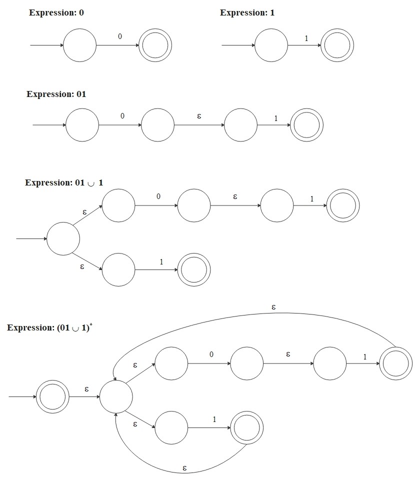
As an example, we convert the regular expression \((01 \cup 1)^*\) into an NFA through a sequence of stages.
The language \(L\bigl((01 \cup 1)^*\bigr)\) consists of strings such as
\[
\{\epsilon, \, 01, \, 1, \, 0101, \, 11, \, 1101, \, 01011101, \, 11111, \, 01101011110111, \, \cdots\}
\]
and the following NFA recognizes this language. When the NFA follows an \(\epsilon\)-transition, it moves to the next state
without reading the next symbol from the input string.
Proof Sketch: Part 2 (DFA → Regex via state elimination)
For the converse direction, suppose \(A\) is regular, so a DFA \(M\) recognizes \(A\). We must produce
a regular expression \(R\) with \(L(R) = A\). The construction proceeds via an intermediate object called
a generalized NFA (GNFA), in which transitions are labeled by regular expressions rather
than single symbols. A GNFA reads input by consuming, on each transition, any string matching that
transition's regex label.
Step 1: Convert \(M\) into a GNFA.
Add a new start state \(s\) with an \(\epsilon\)-edge
to \(M\)'s start state, and a new unique accept state \(t\) with \(\epsilon\)-edges from each of \(M\)'s
accept states. Then ensure that every pair of internal states \((q_i, q_j)\) has exactly one transition
between them (labeled by the union of all symbols that previously triggered \(q_i \to q_j\) in \(M\),
or by the regex \(\emptyset\) if no such symbol existed). The resulting GNFA recognizes exactly \(A\).
Step 2: State elimination.
Repeatedly remove internal states one at a time. To remove
an internal state \(q_{\mathrm{rip}}\), update each remaining transition \(q_i \to q_j\) (for
\(q_i \neq t\) and \(q_j \neq s\)) by replacing its old label \(R_{ij}\) with
\[
R_{ij}^{\text{new}} = R_{ij} \cup R_{i,\mathrm{rip}} \, R_{\mathrm{rip},\mathrm{rip}}^* \, R_{\mathrm{rip},j}
\]
— that is, "either bypass \(q_{\mathrm{rip}}\) entirely (old label), or detour through \(q_{\mathrm{rip}}\)
any number of times before continuing." This new label captures every path that previously went through
\(q_{\mathrm{rip}}\). The Kleene star is essential here: it accounts for self-loops at \(q_{\mathrm{rip}}\)
being traversed any number of times.
Step 3: Read off the regex.
After all internal states are eliminated, only \(s\) and
\(t\) remain, connected by a single transition labeled with some regex \(R\). One can verify that each
elimination step preserves the recognized language, so the final \(R\) satisfies \(L(R) = A\).