Statistical Inference & Hypothesis Testing

Null Hypothesis Significance Test

Once we have a statistical model (or hypothesis), we need to assess whether it is plausible given our data \(\mathcal{D}\). On the MLE page, we developed maximum likelihood estimation as a method for fitting parameters to data. MLE answers the question "what is the best estimate?" but it does not answer a complementary question: "is the effect we observe real, or could it be due to chance?" Hypothesis testing provides a principled framework for making such decisions under uncertainty.

Although Bayesian inference can replace many frequentist techniques and is especially popular in modern machine learning, frequentist methods remain valuable. They are often simpler to compute, more standardized, and provide complementary insights. Here, we introduce the null hypothesis significance test (NHST).

Our reasoning follows the logic of proof by contradiction. If the observed data would be extremely unlikely under \(H_0\), we reject the null hypothesis in favor of \(H_1\). However, rejecting \(H_0\) does not prove \(H_1\) is true, and failing to reject \(H_0\) does not prove \(H_0\) is true. It only means the evidence is insufficient. Because our conclusion can be wrong, we must account for two types of error:

The Type I error rate \(\alpha\) is called the significance level of the test. It represents the probability of mistakenly rejecting \(H_0\) when it is true, and is typically set to 0.05 or 0.01 in practice.

To decide whether to reject \(H_0\), we compute a test statistic \(T(\mathcal{D})\), a function of the data that summarizes the evidence against \(H_0\). We then compare it to the distribution of \(T(\tilde{\mathcal{D}})\) under hypothetical datasets \(\tilde{\mathcal{D}}\) drawn assuming \(H_0\) is true.

The form above is the upper-tailed p-value, appropriate when \(H_1\) predicts larger values of \(T\). The lower-tailed variant replaces \(\geq\) with \(\leq\), and the two-sided version uses \(P(|T(\tilde{\mathcal{D}})| \geq |T(\mathcal{D})|)\) when the test statistic is symmetric under \(H_0\). The choice depends on the alternative hypothesis.

If \(p \lt \alpha\), the observed result is deemed unlikely under \(H_0\), and we reject the null hypothesis. It is essential to interpret p-values correctly. A p-value of 0.05 does not mean that \(H_1\) is true with probability 0.95. The p-value measures the compatibility of the data with \(H_0\), not the probability that \(H_0\) is true or false.

While NHST provides a systematic framework, it has well-known limitations:

• Statistical significance does not imply practical significance. Even if \(H_0\) is rejected, the effect size may be too small to matter.
• p-values depend on sample size. With very large datasets, even tiny, practically irrelevant differences may yield small p-values.
• Bayesian approaches offer an alternative by directly computing the probability of hypotheses given the data, rather than relying on fixed significance thresholds.

To make the NHST framework concrete, we now work through a specific example using the t-test.

t-Tests

The population standard deviation \(\sigma\) is typically unknown in practice. We therefore replace it with the sample standard deviation \(s\) and use the Student's t-distribution instead of the normal distribution. The resulting procedure is called a t-test.

Distributional assumption. If \(n \geq 2\) and \(X_1, \ldots, X_n\) are i.i.d. \(\mathcal{N}(\mu, \sigma^2)\), then the standardized sample mean \((\bar{X} - \mu)/(s/\sqrt{n})\) follows a \(t_{n-1}\) distribution exactly. To see this, note that \(Z := \sqrt{n}(\bar{X} - \mu)/\sigma \sim \mathcal{N}(0,1)\) and \(Q := (n-1)s^2/\sigma^2 \sim \chi^2_{n-1}\), and that \(Z\) and \(Q\) are independent. We take these three facts for granted here. All of them follow from the orthogonal decomposition of a Gaussian sample into its mean and its residuals (Cochran's theorem), which we do not develop. The ratio \(Z/\sqrt{Q/(n-1)} = (\bar{X} - \mu)/(s/\sqrt{n})\) then matches the standard t-distribution definition. For non-normal populations, the result holds only asymptotically via the Central Limit Theorem.

Confidence Intervals vs Credible Intervals

Hypothesis testing gives a binary answer, reject or fail to reject. It says nothing about how close our estimate might be to the true parameter. In practice, we often want a range of plausible values for \(\theta\). Both frequentist and Bayesian statistics provide such intervals, but they differ fundamentally in interpretation.

One subtlety is critical. A 95% CI does not mean "there is a 95% probability that \(\theta\) lies in this interval." In frequentist statistics, \(\theta\) is a fixed constant. It either lies in the interval or it does not. The probability statement refers to the procedure, not to any single interval.

In Bayesian statistics, the interpretation is reversed. The data are fixed (since they are observed) and the parameter is treated as a random variable with a posterior distribution.

Unlike a confidence interval, a credible interval directly states that, given the data and the prior, the parameter falls within the interval with the stated probability.

Example:

Suppose we toss a coin \(n = 100\) times and observe 60 heads. Now we want to estimate the probability of getting heads.

First, we try the frequentist approach. The point estimate for the probability of heads \(p\) is \(\hat{p} = \frac{60}{100} = 0.6\), and the standard error (SE) for a proportion is given by: \[ \begin{align*} \operatorname{SE} &= \sqrt{\frac{\hat{p}(1-\hat{p})}{n}} \\\\ &= \sqrt{\frac{0.6 \times 0.4}{100}} \\\\ &\approx 0.049. \end{align*} \]

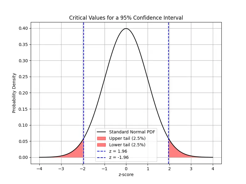
For a 95% CI using normal approximation, the critical value is \(z_{0.025} \approx 1.96\). Then the CI is given by \[ \begin{align*} \operatorname{CI} &= [\hat{p}-z_{0.025} \times \operatorname{SE}, \quad \hat{p}+z_{0.025}\times \operatorname{SE}] \\\\ &\approx [0.504, 0.696]. \end{align*} \] If we repeated the experiment (tossing the coin 100 times) many times and computed a 95% CI each time, about 95% of the resulting intervals would cover the true \(p\).

Note. A z-score is any value that has been standardized to represent the number of standard deviations away from the mean. The critical value is a specific z-score used as a threshold in hypothesis testing or confidence interval calculations. In our case, \(z_{0.025} \approx 1.96\) is the critical value that separates the central 95% of the distribution from the outer 5% (2.5% in each tail).

In the Bayesian approach, we assume a uniform prior for the probability \(p\), which is equivalent to a Beta distribution: \[ p \sim \operatorname{Beta}(1, 1). \]

With 60 heads and 40 tails, the likelihood is given by a binomial distribution. In the Bayesian framework, the posterior distribution is: \[ p \sim \operatorname{Beta}(1+60, 1+40) = \operatorname{Beta}(61, 41). \]

Note. The Beta distribution is a conjugate prior for the binomial likelihood. Because the likelihood for coin tosses is binomial, a Beta prior yields a Beta posterior.

A 95% credible interval (CrI) is typically obtained by finding the 2.5th and 97.5th percentiles of the posterior distribution. These percentiles can be computed using the inverse cumulative distribution function for the Beta distribution. For example, \[ \begin{align*} \operatorname{CrI} &= [\operatorname{invBeta}(0.025, 61, 41), \quad \operatorname{invBeta}(0.975, 61, 41)] \\\\ &\approx [0.50, 0.69]. \end{align*} \]

Given the observed data and the chosen prior, there is a 95% probability that \(p\) falls between 0.50 and 0.69. This interval directly reflects our uncertainty about \(p\) after seeing the data.

The credible interval is often considered more intuitive, because it directly answers the question "What is the probability that the parameter falls within this interval, given the data and our prior beliefs?" Frequentist methods, on the other hand, provide guarantees on long-run performance without the need for a prior, which can be an advantage in settings where subjective beliefs are hard to justify.

Bootstrap

The confidence intervals derived above rely on distributional assumptions. The usual assumption is that the sampling distribution is approximately normal by the Central Limit Theorem. These analytical approximations may be unreliable when the sample size is small, when the estimator is a complex function of the data, or when the underlying distribution is far from normal. The bootstrap method provides a powerful non-parametric alternative, although its own justification is also asymptotic. This procedure is motivated by the Glivenko-Cantelli theorem, which guarantees that the empirical cdf converges uniformly to the true cdf almost surely as the sample size grows.

The idea is conceptually simple. We treat the observed sample as a proxy for the population and resample from it with replacement to generate many bootstrap samples. By computing the estimator on each bootstrap sample, we obtain an empirical approximation of the estimator's sampling distribution. This approach provides a flexible, non-parametric way to assess uncertainty and construct confidence intervals.

Example:

We have a small dataset of 10 people's heights (in cm): \[ x = [160,165,170,175,180,185,190,195,200,205]. \] The sample mean is \(\hat{\mu} = 182.5\). Since our sample size is small, we might not be able to assume the sampling distribution of the mean is normal. Instead of assuming normality, we use bootstrap resampling to approximate it empirically.

Here, we randomly draw 10 values from the original sample with replacement. Some values may be repeated, and others may be missing in a given resample. For example, we might obtain: \[ \begin{align*} &x_1 = [165,175,175,190,185,160,200,195,180,185], \\\\ &\hat{\mu} = 181.0. \end{align*} \]

Then we repeat this process many times (for example, 10,000 times). Each time, we create a new resampled dataset, compute its mean, and store it. Once we have 10,000 bootstrap sample means, we can use them to estimate the confidence interval.

With the tools for estimation (MLE) and inference (hypothesis testing, confidence intervals) established, we can now apply them to one of the most important models in statistics. On the linear regression page, we develop linear regression as the intersection of least-squares optimization and maximum likelihood estimation under Gaussian noise.