Bayesian Decision Theory

Introduction

In Part 14, we introduced Bayesian inference and derived posterior distributions for unknown parameters. In Part 18, we developed Markov chains for modeling sequential data, noting that Markov Chain Monte Carlo (MCMC) methods use the Markov property to sample from complex posterior distributions.

So far, our development of Bayesian statistics has focused on inference: given observed data, how should we update our beliefs about unknown quantities? But inference alone does not tell us what to do. In many applications - medical diagnosis, spam filtering, autonomous driving - we must ultimately choose an action based on uncertain information. Bayesian decision theory provides the principled framework for making such optimal decisions under uncertainty.

The setup is as follows. An agent must choose an action \(a\) from a set of possible actions \(\mathcal{A}\). The consequence of this action depends on the unknown state of nature \(h \in \mathcal{H}\), which the agent cannot observe directly. To quantify the cost of choosing an action \(a\) when the true state is \(h\), we introduce a loss function \(l(h, a)\).

The key idea of Bayesian decision theory is to combine the loss function with the posterior distribution \(p(h \mid \boldsymbol{x})\) obtained from observed evidence \(\boldsymbol{x}\) (or a dataset \(\mathcal{D}\)). For any action \(a\), the posterior expected loss (or posterior risk) is defined as follows.

A rational agent should select the action that minimizes this expected loss. This leads to the central concept of the section.

Equivalently, by defining the utility function \(U(h, a) = -l(h, a)\), which measures the desirability of each action in each state, the Bayes estimator can be written as \[ \pi^*(\boldsymbol{x}) = \arg \max_{a \in \mathcal{A}} \, \mathbb{E}_{h}[U(h, a)]. \] This utility-maximization formulation is natural in economics, game theory, and reinforcement learning, where the focus is on maximizing expected rewards rather than minimizing losses.

The power of this framework lies in its generality: by choosing different loss functions, we recover many familiar estimators and decision rules as special cases. We begin with the most common setting in machine learning - classification under zero-one loss.

Classification (Zero-One Loss)

Perhaps the most common application of Bayesian decision theory in machine learning is classification: given an input \(\boldsymbol{x} \in \mathcal{X}\), we wish to assign it the optimal class label. To apply the general framework, we specify the states, actions, and loss function for this particular setting.

Suppose that the states of nature correspond to class labels \[ \mathcal{H} = \mathcal{Y} = \{1, \ldots, C\}, \] and that the possible actions are also the class labels: \(\mathcal{A} = \mathcal{Y}\). A natural loss function in this context is the zero-one loss, which penalizes misclassification equally regardless of which classes are confused.

Under the zero-one loss, the posterior expected loss for choosing label \(\hat{y}\) becomes \[ \rho(\hat{y} \mid \boldsymbol{x}) = p(\hat{y} \neq y^* \mid \boldsymbol{x}) = 1 - p(y^* = \hat{y} \mid \boldsymbol{x}). \] Thus, minimizing the expected loss is equivalent to maximizing the posterior probability: \[ \pi^*(\boldsymbol{x}) = \arg \max_{y \in \mathcal{Y}} \, p(y \mid \boldsymbol{x}). \] In other words, the optimal decision under zero-one loss is to select the mode of the posterior distribution, which is the maximum a posteriori (MAP) estimate. This provides a decision-theoretic justification for the MAP estimator that we encountered in Part 14.

The Reject Option

In some scenarios - particularly safety-critical applications such as medical diagnosis or autonomous driving - the cost of an incorrect classification may be so high that it is preferable for the system to abstain from making a decision when it is uncertain. This is formalized through the reject option.

Under this approach, the set of available actions is expanded to include a reject action: \[ \mathcal{A} = \mathcal{Y} \cup \{0\}, \] where action \(0\) represents the reject option (i.e., saying "I'm not sure"). The loss function is then defined as \[ l(y^*, a) = \begin{cases} 0 & \text{if } y^* = a \text{ and } a \in \{1, \ldots, C\} \\ \lambda_r & \text{if } a = 0 \\ \lambda_e & \text{otherwise} \end{cases} \] where \(\lambda_r\) is the cost of the reject action and \(\lambda_e\) is the cost of a classification error. For the reject option to be meaningful, we require \(0 < \lambda_r < \lambda_e\); otherwise, rejecting is either free (and we would always reject) or more expensive than guessing (and we would never reject).

Under this framework, instead of always choosing the label with the highest posterior probability, the optimal policy chooses a label only when the classifier is sufficiently confident: \[ a^* = \begin{cases} y^* & \text{if } p^* > \lambda^* \\ \text{reject} & \text{otherwise} \end{cases} \] where \[ p^* = \max_{y \in \{1, \ldots, C\}} p(y \mid \boldsymbol{x}), \qquad \lambda^* = 1 - \frac{\lambda_r}{\lambda_e}. \]

Confusion Matrix

The Bayes estimator tells us what the optimal decision rule is, but in practice, we need to measure how well a classifier actually performs on real data. The standard tool for this is the (class) confusion matrix, which provides a complete summary of the outcomes of classification decisions. We recall the four possible outcomes from Part 10: Statistical Inference & Hypothesis Testing, where we first introduced Type I and Type II errors.

For binary classification (\(y \in \{0, 1\}\)), each prediction falls into one of four categories:

• True Positives (TP): instances correctly classified as positive.
• True Negatives (TN): instances correctly classified as negative.
• False Positives (FP): instances incorrectly classified as positive (Type I error).
• False Negatives (FN): instances incorrectly classified as negative (Type II error).

Understanding the distinction between FP and FN is critical because the costs associated with each error type may differ significantly depending on the application. In safety-critical systems, a false negative (missing a dangerous condition) is typically far more costly than a false positive (raising an unnecessary alarm). For example, in medical screening, a false positive means unnecessarily alarming a healthy patient, whereas a false negative means failing to detect a disease in someone who needs treatment.

In the context of Bayesian decision theory, the confusion matrix quantifies the empirical performance of the Bayes estimator (or any other decision rule) by counting how often the predicted labels match or mismatch the true labels.

In practice, a binary classifier typically outputs a probability \(p(y = 1 \mid \boldsymbol{x})\), and the final prediction depends on a decision threshold \(\tau \in [0, 1]\). For any fixed threshold \(\tau\), the decision rule is \[ \hat{y}_{\tau}(\boldsymbol{x}) = \mathbb{I}\left(p(y = 1 \mid \boldsymbol{x}) \geq \tau\right). \] Given a set of \(N\) labeled examples, we can compute the empirical counts for each cell of the confusion matrix. For example, \[ \begin{align*} \text{FP}_{\tau} &= \sum_{n=1}^N \mathbb{I}(\hat{y}_{\tau}(\boldsymbol{x}_n) = 1, \, y_n = 0),\\\\ \text{FN}_{\tau} &= \sum_{n=1}^N \mathbb{I}(\hat{y}_{\tau}(\boldsymbol{x}_n) = 0, \, y_n = 1). \end{align*} \]

Since the confusion matrix depends on the choice of \(\tau\), different thresholds lead to different trade-offs between error types. How should we choose \(\tau\), and how can we evaluate a classifier's performance across all possible thresholds? This motivates the ROC and PR curves developed in the following sections.

Receiver Operating Characteristic Curves

Rather than evaluating a classifier at a single threshold, we can characterize its performance across all thresholds simultaneously. The receiver operating characteristic (ROC) curve achieves this by plotting two rates derived from the confusion matrix. To obtain these rates, we normalize the confusion matrix per row, yielding the conditional distribution \(p(\hat{y} \mid y)\). Since each row sums to 1, these rates describe the classifier's behavior separately within the positive and negative populations.

• True positive rate (TPR) (or Sensitivity / Recall): \[ \text{TPR}_{\tau} = p(\hat{y} = 1 \mid y = 1, \tau) = \frac{\text{TP}_{\tau}}{\text{TP}_{\tau} + \text{FN}_{\tau}}. \]
• False positive rate (FPR) (or Type I error rate / Fallout): \[ \text{FPR}_{\tau} = p(\hat{y} = 1 \mid y = 0, \tau) = \frac{\text{FP}_{\tau}}{\text{FP}_{\tau} + \text{TN}_{\tau}}. \]
• False negative rate (FNR) (or Type II error rate / Miss rate):\[ \text{FNR}_{\tau} = p(\hat{y} = 0 \mid y = 1, \tau) = \frac{\text{FN}_{\tau}}{\text{TP}_{\tau} + \text{FN}_{\tau}}. \]
• True negative rate (TNR) (or Specificity):\[ \text{TNR}_{\tau} = p(\hat{y} = 0 \mid y = 0, \tau) = \frac{\text{TN}_{\tau}}{\text{FP}_{\tau} + \text{TN}_{\tau}}. \]

By plotting TPR against FPR as an implicit function of \(\tau\), we obtain the ROC curve. The overall quality of a classifier is often summarized using the AUC (Area Under the Curve). A higher AUC indicates better discriminative ability across all threshold values, with a maximum of 1.0 for a perfect classifier.

The figure below compares two classifiers — one trained using logistic regression and the other using a random forest. Both classifiers provide predicted probabilities for the positive class, allowing us to vary \(\tau\) and compute the corresponding TPR and FPR. A diagonal line is also drawn, representing the performance of a random classifier — i.e., one that assigns labels purely by chance. On this line, the TPR equals the FPR at every threshold. If a classifier's ROC curve lies on this diagonal, it means the classifier is performing no better than random guessing. In contrast, any performance above the diagonal indicates that the classifier is capturing some signal, while performance below the diagonal (rare in practice) would indicate worse-than-random behavior.

In our demonstration, the logistic regression model has been intentionally made worse, yielding an AUC of 0.78, while the random forest shows superior performance with an AUC of 0.94. These results mean that, overall, the random forest is much better at distinguishing between the positive and negative classes compared to the underperforming logistic regression model.

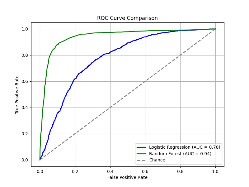
(Data: 10,000 samples, 20 total features, 5 features are informative, 2 clusters per class, 5% label noise.)

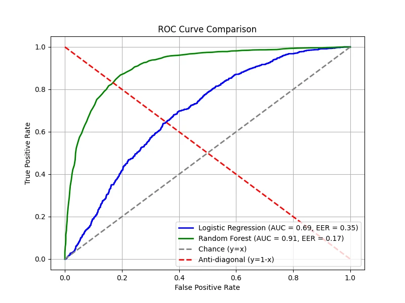
Equal Error Rate (EER)

The ROC curve provides a comprehensive view of the trade-off between TPR and FPR, but it can be useful to summarize this trade-off with a single number. The equal error rate (EER) is the operating point where \(\text{FPR} = \text{FNR}\). This point represents the optimal threshold under the assumption that the prior probabilities and the costs of both types of errors are equal. This metric is particularly important in applications such as biometric authentication (fingerprint or face recognition), where false acceptance and false rejection carry comparable costs.

The figure below shows the EER point for our two models, marking where the FPR and FNR curves intersect:

A perfect classifier would achieve an EER of 0, corresponding to the top-left corner of the ROC curve. In practice, one may tune the decision threshold to operate at or near the EER, depending on the application's requirements.

The ROC curve and EER evaluate a classifier by conditioning on the true class (i.e., how the classifier behaves within each population). However, in many practical settings we care about a different question: given that the classifier predicted positive, how likely is it to be correct? This leads us to precision-recall analysis.

Precision-Recall (PR) Curves

Here, we normalize the confusion matrix per column to obtain \(p(y \mid \hat{y})\), which conditions on the predicted label. The column-normalized confusion matrix answers a complementary question: among the instances predicted as positive (or negative), what fraction are truly positive (or negative)? This perspective is especially important when precision is critical, such as in medical diagnosis or fraud detection.

• Positive predictive value (PPV) (or Precision):\[ \text{PPV}_{\tau} = p(y = 1 \mid \hat{y} = 1, \tau) = \frac{\text{TP}_{\tau}}{\text{TP}_{\tau} + \text{FP}_{\tau}}. \]
• False discovery rate (FDR):\[ \text{FDR}_{\tau} = p(y = 0 \mid \hat{y} = 1, \tau) = \frac{\text{FP}_{\tau}}{\text{TP}_{\tau} + \text{FP}_{\tau}}. \]
• False omission rate (FOR):\[ \text{FOR}_{\tau} = p(y = 1 \mid \hat{y} = 0, \tau) = \frac{\text{FN}_{\tau}}{\text{FN}_{\tau} + \text{TN}_{\tau}}. \]
• Negative predictive value (NPV):\[ \text{NPV}_{\tau} = p(y = 0 \mid \hat{y} = 0, \tau) = \frac{\text{TN}_{\tau}}{\text{FN}_{\tau} + \text{TN}_{\tau}}. \]

Note that within each column, the rates sum to 1: \(\text{PPV} + \text{FDR} = 1\) and \(\text{FOR} + \text{NPV} = 1\).

To summarize a system's performance - especially when classes are imbalanced (i.e., when the positive class is rare) or when false positives and false negatives have different costs - we often use a precision-recall (PR) curve. This curve plots precision against recall as the decision threshold \(\tau\) varies.

Imbalanced datasets appear frequently in real-world machine learning applications where one class is naturally much rarer than the other. For example, in financial transactions, fraudulent activities are rare compared to legitimate ones. The classifier must detect the very few fraud cases (positive class) among millions of normal transactions (negative class).

Let precision be \(\mathcal{P}(\tau)\) and recall be \(\mathcal{R}(\tau)\). If \(\hat{y}_n \in \{0, 1\}\) is the predicted label and \(y_n \in \{0, 1\}\) is the true label, then at threshold \(\tau\), precision and recall can be estimated by: \[ \mathcal{P}(\tau) = \frac{\sum_n y_n \hat{y}_n}{\sum_n \hat{y}_n}, \quad \mathcal{R}(\tau) = \frac{\sum_n y_n \hat{y}_n}{\sum_n y_n}. \] By plotting the precision vs recall for various the threshold \(\tau\), we obtain the PR curve.

This curve visually represents the trade-off between precision and recall. It is particularly valuable in situations where one class is much rarer than the other or when false alarms carry a significant cost.

A crucial difference between the ROC and PR curves is the baseline for a random classifier. While a random classifier always yields an AUC of 0.5 on an ROC curve, the baseline for a PR curve is the fraction of positive samples in the dataset: \[ y_{baseline} = \frac{P}{P + N} \] This makes the PR curve a much more rigorous evaluation tool for highly imbalanced datasets, as the "no-knowledge" score can be near zero while the "perfect" score remains 1.0.

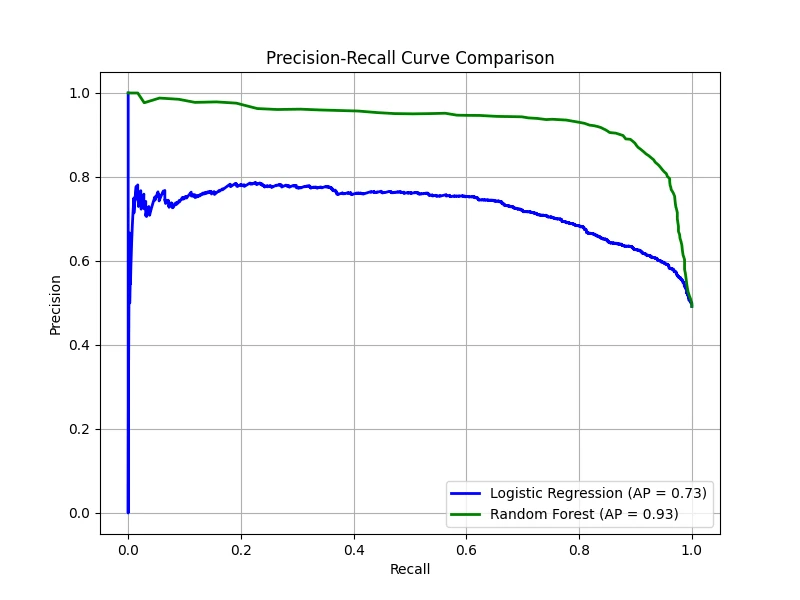
However, raw precision values can be noisy as the threshold varies. To stabilize this, interpolated precision is often computed. For a given recall level \(r\), it is defined as the maximum precision observed for any recall level greater than or equal to \(r\): \[ \mathcal{P}_{\text{interp}}(r) = \max_{r' \geq r} \mathcal{P}(r') \] The average precision (AP) is the area under this interpolated PR curve. It provides a single-number summary that reflects the classifier's ability to maintain high precision as the recall threshold is lowered.

In our case, the logistic regression produced an AP of 0.73, while the random forest achieved a much stronger AP of 0.93. This indicates that the random forest is significantly more robust at identifying positive cases without sacrificing precision.

Note: In settings where multiple PR curves are generated (for example, one for each query in information retrieval or one per class in multi-class classification), the mean average precision (mAP) is computed as the mean of the AP scores over all curves. mAP offers an overall performance measure across multiple queries or classes.

Class Imbalance

In real-world applications, the class distribution is far from uniform. A dataset is considered imbalanced when one class has significantly fewer examples than the other - for instance, 5% positive samples and 95% negative samples. In such cases, naive metrics like accuracy can be highly misleading: a model that always predicts the majority class achieves high accuracy without correctly identifying any minority class instances. How do ROC-AUC and PR-AP behave differently under class imbalance?

The ROC-AUC metric is often insensitive to class imbalance because both TPR and FPR are computed within their respective populations - TPR is a ratio within the positive samples and FPR is a ratio within the negative samples. Consequently, the class proportions do not directly affect the ROC curve.

On the other hand, the PR-AP metric is more sensitive to class imbalance. This is because precision depends on both populations: \[ \text{Precision} = \frac{\text{TP}}{\text{TP} + \text{FP}}. \] When the negative class vastly outnumbers the positive class, even a small false positive rate can produce a large absolute number of false positives, significantly reducing precision.

To demonstrate this effect, we create a dataset where 90% of the samples belong to the negative class and only 10% belong to the positive class, then train both the logistic regression and random forest models again:

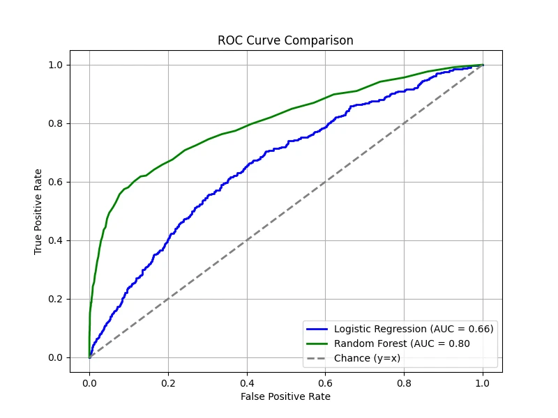
ROC Curve (Imbalanced)

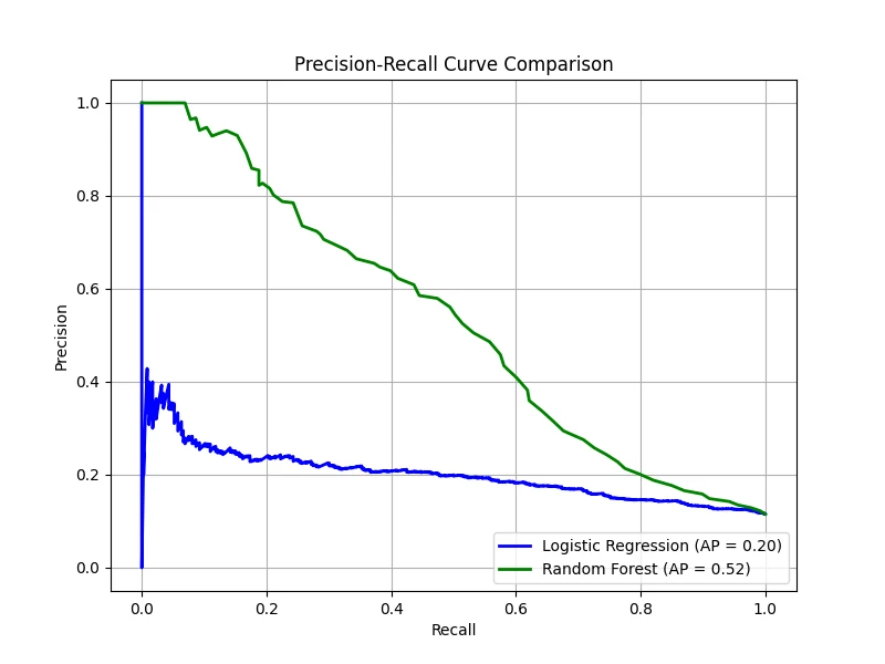
Precision-Recall Curve (Imbalanced)

The ROC curves remain relatively smooth and the AUC does not drop drastically, even though the dataset is highly imbalanced. The PR curves, however, reveal a distinct difference, with noticeably lower AP scores. This highlights how class imbalance makes it harder to achieve high precision and recall simultaneously. Even though the random forest outperforms logistic regression, it still struggles to detect the rare positive cases effectively.

In summary, PR curves focus on precision and recall, which directly reflect how well a model identifies the minority class. Precision, in particular, is sensitive to even a small number of false positives, providing a more realistic picture of performance when the positive class is scarce. Thus, PR-AP is generally the preferred metric for imbalanced classification problems because it directly measures performance on the minority class.