Support Vector Machine
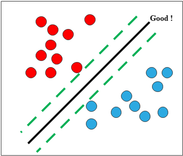
So far in both regression and classification, we have used probabilistic predictors that model \(p(y \mid \mathbf{x})\) and optimize via maximum likelihood. Here, we take a fundamentally different, geometric approach: rather than modeling probabilities, we seek the hyperplane that separates the classes with the largest possible margin. This formulation leads naturally to a constrained optimization problem whose dual formulation enables the kernel trick.
This margin-based approach often leads to strong generalization, especially in high dimensional spaces with limited samples. By employing the kernel trick (e.g., RBF kernel), SVMs can implicitly map inputs into higher dimensional feature spaces, enabling the classification of nonlinearly separable data without explicitly computing those transformations. Despite the rise of deep learning, SVMs remain valuable for small- to medium-sized datasets, offering robustness and interpretability through a sparse set of support vectors.
In binary classification with labels \(\tilde{y} \in \{-1, +1\}\), the prediction is \(h(\mathbf{x}) = \operatorname{sign}(f(\mathbf{x}))\), and the decision boundary (hyperplane) is defined by \[ f(\mathbf{x}) = \mathbf{w}^\top \mathbf{x} + b. \tag{1} \] To obtain a robust solution, we would like to maximize the margin between data points and the decision boundary.
To express the distance of the closest point to the decision boundary, we decompose any point \(\mathbf{x}\) as its orthogonal projection onto the hyperplane \(H = \{\mathbf{x} : f(\mathbf{x}) = 0\}\) plus a signed normal component: \[ \mathbf{x} = \operatorname{proj}_H \mathbf{x} + r \frac{\mathbf{w}}{\|\mathbf{w}\|}, \tag{2} \] where \(r\) is the signed distance from \(\mathbf{x}\) to \(H\), and \(\mathbf{w}/\|\mathbf{w}\|\) is the unit normal vector to \(H\).
Substituting Expression (2) into the boundary function (1): \[ \begin{align*} f(\mathbf{x}) &= \mathbf{w}^\top \!\left(\operatorname{proj}_H \mathbf{x} + r \frac{\mathbf{w}}{\|\mathbf{w}\|}\right) + b \\\\ &= \underbrace{\mathbf{w}^\top \operatorname{proj}_H \mathbf{x} + b}_{= \, f(\operatorname{proj}_H \mathbf{x}) \, = \, 0} + r \|\mathbf{w}\| \\\\ &= r \|\mathbf{w}\|. \end{align*} \] Hence \[ r = \frac{f(\mathbf{x})}{\|\mathbf{w}\|}, \] and each correctly classified point satisfies \[ \tilde{y}_n f(\mathbf{x}_n) > 0. \] Therefore, our objective is \[ \max_{\mathbf{w},\, b} \frac{1}{\|\mathbf{w}\|} \min_{1 \leq n \leq N} \tilde{y}_n \!\left(\mathbf{w}^\top \mathbf{x}_n + b\right). \] Since both \(\mathbf{w}\) and \(b\) can be freely rescaled without changing the decision boundary, we may normalize so that the closest point satisfies \(\tilde{y}_n f(\mathbf{x}_n) = 1\) exactly. Under this normalization, the margin (distance between the two parallel supporting hyperplanes) equals \(\frac{2}{\|\mathbf{w}\|}\).
Note that \(\max \frac{1}{\|\mathbf{w}\|}\) is equivalent to \(\min \|\mathbf{w}\|^2\). Thus our objective becomes:
\[ \min_{\mathbf{w},\, b} \;\frac{1}{2}\|\mathbf{w}\|^2 \] subject to \[ \tilde{y}_n(\mathbf{w}^\top \mathbf{x}_n + b) \geq 1, \quad n = 1, \ldots, N. \] The factor of \(\frac{1}{2}\) is included for convenience when differentiating.
This constrained optimization problem, known as the primal problem, is difficult to solve directly. Since the objective is convex and the inequality constraints are linear, Slater's condition is automatically satisfied, so strong duality holds and the problem can equivalently be solved via its dual, which often has computational advantages and enables the kernel trick.
Let \(\boldsymbol{\alpha} \in \mathbb{R}^N\) be the vector of Lagrange multipliers associated with the inequality constraints. The Lagrangian is \[ \mathcal{L}(\mathbf{w}, b, \boldsymbol{\alpha}) = \frac{1}{2}\mathbf{w}^\top \mathbf{w} - \sum_{n=1}^N \alpha_n \!\left(\tilde{y}_n (\mathbf{w}^\top \mathbf{x}_n + b) - 1\right). \tag{3} \] A primal-dual optimum \((\hat{\mathbf{w}}, \hat{b}, \hat{\boldsymbol{\alpha}})\) satisfies \[ (\hat{\mathbf{w}}, \hat{b}, \hat{\boldsymbol{\alpha}}) = \min_{\mathbf{w}, b} \max_{\boldsymbol{\alpha} \geq \mathbf{0}} \mathcal{L}(\mathbf{w}, b, \boldsymbol{\alpha}). \] Taking derivatives with respect to \(\mathbf{w}\) and \(b\) and setting them to zero (the stationarity condition): \[ \begin{align*} \nabla_{\mathbf{w}} \mathcal{L} &= \mathbf{w} - \sum_{n=1}^N \alpha_n \tilde{y}_n \mathbf{x}_n = \mathbf{0}, \\\\ \frac{\partial \mathcal{L}}{\partial b} &= -\sum_{n=1}^N \alpha_n \tilde{y}_n = 0, \end{align*} \] which gives \[ \begin{align*} \hat{\mathbf{w}} &= \sum_{n=1}^N \hat{\alpha}_n \tilde{y}_n \mathbf{x}_n, \\\\ 0 &= \sum_{n=1}^N \hat{\alpha}_n \tilde{y}_n. \end{align*} \] Substituting these into the Lagrangian (3): \[ \begin{align*} \mathcal{L}(\hat{\mathbf{w}}, \hat{b}, \boldsymbol{\alpha}) &= \frac{1}{2}\hat{\mathbf{w}}^\top \hat{\mathbf{w}} - \sum_{n=1}^N \alpha_n \tilde{y}_n \hat{\mathbf{w}}^\top \mathbf{x}_n - \hat{b} \sum_{n=1}^N \alpha_n \tilde{y}_n + \sum_{n=1}^N \alpha_n \\\\ &= \frac{1}{2}\hat{\mathbf{w}}^\top \hat{\mathbf{w}} - \hat{\mathbf{w}}^\top \hat{\mathbf{w}} - 0 + \sum_{n=1}^N \alpha_n \\\\ &= \sum_{n=1}^N \alpha_n - \frac{1}{2} \sum_{i=1}^N \sum_{j=1}^N \alpha_i \alpha_j \tilde{y}_i \tilde{y}_j \, \mathbf{x}_i^\top \mathbf{x}_j. \end{align*} \]
\[ \max_{\boldsymbol{\alpha}} \;\sum_{n=1}^N \alpha_n - \frac{1}{2} \sum_{i=1}^N \sum_{j=1}^N \alpha_i \alpha_j \tilde{y}_i \tilde{y}_j \, \mathbf{x}_i^\top \mathbf{x}_j \] subject to \[ \sum_{n=1}^N \alpha_n \tilde{y}_n = 0, \qquad \alpha_n \geq 0, \quad n = 1, \ldots, N. \] The primal-dual solution must satisfy the KKT conditions: \[ \begin{align*} \mathbf{w} - \sum_{n=1}^N \alpha_n \tilde{y}_n \mathbf{x}_n &= \mathbf{0}, \quad \sum_{n=1}^N \alpha_n \tilde{y}_n = 0 &&\text{(stationarity)} \\\\ \tilde{y}_n f(\mathbf{x}_n) - 1 &\geq 0 &&\text{(primal feasibility)} \\\\ \alpha_n &\geq 0 &&\text{(dual feasibility)} \\\\ \alpha_n (\tilde{y}_n f(\mathbf{x}_n) - 1) &= 0 &&\text{(complementary slackness)} \end{align*} \]
Complementary slackness implies that, for each data point, either \[ \alpha_n = 0 \quad \text{or} \quad \tilde{y}_n (\hat{\mathbf{w}}^\top \mathbf{x}_n + \hat{b}) = 1. \] The points satisfying the second condition are called support vectors.
Let the set of support vectors be \(\mathcal{S}\). To perform prediction, we expand \(\hat{\mathbf{w}} = \sum_{n \in \mathcal{S}} \hat{\alpha}_n \tilde{y}_n \mathbf{x}_n\): \[ \begin{align*} f(\mathbf{x};\, \hat{\mathbf{w}}, \hat{b}) &= \hat{\mathbf{w}}^\top \mathbf{x} + \hat{b} \\\\ &= \sum_{n \in \mathcal{S}} \hat{\alpha}_n \tilde{y}_n\, \mathbf{x}_n^\top \mathbf{x} + \hat{b}. \end{align*} \] By the kernel trick, the inner product can be replaced with a positive definite kernel \(\mathcal{K}(\mathbf{x}, \mathbf{x}') = \langle \phi(\mathbf{x}), \phi(\mathbf{x}') \rangle\), implicitly mapping inputs to a higher- (or infinite-) dimensional feature space without ever computing \(\phi\) explicitly.
\[ f(\mathbf{x}) = \sum_{n \in \mathcal{S}} \hat{\alpha}_n \tilde{y}_n \mathcal{K}(\mathbf{x}_n, \mathbf{x}) + \hat{b}, \] where the bias is computed by averaging over the support vectors: \[ \begin{align*} \hat{b} &= \frac{1}{|\mathcal{S}|} \sum_{n \in \mathcal{S}} \!\left(\tilde{y}_n - \hat{\mathbf{w}}^\top \mathbf{x}_n \right) \\\\ &= \frac{1}{|\mathcal{S}|} \sum_{n \in \mathcal{S}} \!\left(\tilde{y}_n - \sum_{m \in \mathcal{S}} \hat{\alpha}_m \tilde{y}_m \mathbf{x}_m^\top \mathbf{x}_n \right). \end{align*} \] Applying the kernel trick to the bias as well: \[ \hat{b} = \frac{1}{|\mathcal{S}|} \sum_{n \in \mathcal{S}} \!\left(\tilde{y}_n - \sum_{m \in \mathcal{S}} \hat{\alpha}_m \tilde{y}_m \mathcal{K}(\mathbf{x}_m, \mathbf{x}_n) \right). \]