Graph Laplacian Fundamentals
Throughout Section I, we have built up the vocabulary of linear algebra —
vector spaces,
linear transformations,
eigendecompositions,
symmetric matrices and their
spectral theorem,
and more specialized tools like the trace and matrix norms,
the Kronecker product, and
stochastic matrices. These tools were developed
in the abstract, on \(\mathbb{R}^n\) or \(M_n(\mathbb{R})\) with no particular geometric
context. The question now becomes: what happens when we apply them to a space
that carries genuine combinatorial structure?
Graphs are the simplest such structure — a finite set of nodes equipped with
pairwise relations. To apply the spectral machinery we have built, we need a matrix that
faithfully encodes a graph's connectivity. The graph Laplacian is
exactly this matrix. It captures how "different" adjacent vertices are from each other,
making it the natural bridge between
graph theory and the
spectral methods we have spent Section I developing. The bridge turns out to be
remarkably rich: a single matrix, defined in two lines, will give us connectivity,
clustering, frequency analysis, and diffusion — all from its eigenstructure.
Definition: Unnormalized Graph Laplacian
For a graph \(G\) with adjacency matrix \(\boldsymbol{A}\) and degree matrix \(\boldsymbol{D}\),
the unnormalized graph Laplacian is the matrix
\[
\boldsymbol{L} = \boldsymbol{D} - \boldsymbol{A}.
\]
Its entries are given by
\[
L_{ij} = \begin{cases} \deg(v_i) & \text{if } i = j \\ -1 & \text{if } i \neq j \text{ and } v_i \sim v_j \\ 0 & \text{otherwise} \end{cases}
\]
where \(v_i \sim v_j\) means vertices \(v_i\) and \(v_j\) are adjacent.
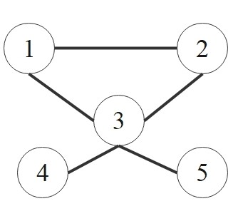
Example:
\[
\underbrace{
\begin{bmatrix} 2 & 0 & 0 & 0 & 0 \\
0 & 2 & 0 & 0 & 0 \\
0 & 0 & 4 & 0 & 0 \\
0 & 0 & 0 & 1 & 0 \\
0 & 0 & 0 & 0 & 1 \\
\end{bmatrix}
}_{\boldsymbol{D}}
-
\underbrace{
\begin{bmatrix} 0 & 1 & 1 & 0 & 0 \\
1 & 0 & 1 & 0 & 0 \\
1 & 1 & 0 & 1 & 1 \\
0 & 0 & 1 & 0 & 0 \\
0 & 0 & 1 & 0 & 0 \\
\end{bmatrix}
}_{\boldsymbol{A}}
=
\underbrace{
\begin{bmatrix} 2 & -1 & -1 & 0 & 0 \\
-1 & 2 & -1 & 0 & 0 \\
-1 & -1 & 4 & -1 & -1 \\
0 & 0 & -1 & 1 & 0 \\
0 & 0 & -1 & 0 & 1 \\
\end{bmatrix}
}_{\boldsymbol{L}}
\]
The Laplacian Quadratic Form (Measuring Smoothness)
The definition \(\boldsymbol{L} = \boldsymbol{D} - \boldsymbol{A}\) may appear
arbitrary, but the Laplacian has a natural interpretation through its quadratic form,
which measures how much a signal varies across the edges of the graph.
Theorem: Dirichlet Energy
For any signal \(\boldsymbol{f} \in \mathbb{R}^n\) defined on the vertices of a
graph with Laplacian \(\boldsymbol{L}\), the quadratic form satisfies
\[
\boldsymbol{f}^\top \boldsymbol{L} \boldsymbol{f} = \sum_{(i,j) \in E} w_{ij}(f_i - f_j)^2
\]
where \(w_{ij}\) is the weight of edge \((i,j)\) (equal to 1 for unweighted graphs).
This quantity is called the Dirichlet energy of \(\boldsymbol{f}\).
Proof:
We work with the weighted adjacency matrix \(\boldsymbol{A} = (w_{ij})\), where
\(w_{ij} = w_{ji} \geq 0\) and \(w_{ij} = 0\) when \(v_i \not\sim v_j\) (the unweighted
case is \(w_{ij} \in \{0, 1\}\)). The weighted degree is \(d_i = \sum_{j} w_{ij}\),
and \(\boldsymbol{L} = \boldsymbol{D} - \boldsymbol{A}\).
Split the quadratic form:
\[
\boldsymbol{f}^\top \boldsymbol{L} \boldsymbol{f}
= \boldsymbol{f}^\top \boldsymbol{D} \boldsymbol{f} - \boldsymbol{f}^\top \boldsymbol{A} \boldsymbol{f}
= \sum_{i} d_i f_i^2 - \sum_{i,j} w_{ij} f_i f_j.
\]
Rewrite the degree term using \(d_i = \sum_{j} w_{ij}\), then symmetrize via
\(w_{ij} = w_{ji}\):
\[
\sum_{i} d_i f_i^2
= \sum_{i,j} w_{ij} f_i^2
= \tfrac{1}{2}\sum_{i,j} w_{ij} f_i^2 + \tfrac{1}{2}\sum_{i,j} w_{ij} f_j^2
= \tfrac{1}{2}\sum_{i,j} w_{ij} (f_i^2 + f_j^2),
\]
where the second sum in the middle expression is obtained from the first by swapping
the dummy indices \(i \leftrightarrow j\) (which is free to do) and then using
\(w_{ji} = w_{ij}\). Now substitute into the split, writing the second term as
\(\sum_{i,j} w_{ij} f_i f_j = \tfrac{1}{2}\sum_{i,j} w_{ij}(2 f_i f_j)\) so that both
terms share the prefactor \(\tfrac{1}{2}\):
\[
\boldsymbol{f}^\top \boldsymbol{L} \boldsymbol{f}
= \tfrac{1}{2}\sum_{i,j} w_{ij}(f_i^2 + f_j^2) - \tfrac{1}{2}\sum_{i,j} w_{ij}(2 f_i f_j)
= \tfrac{1}{2}\sum_{i,j} w_{ij}(f_i - f_j)^2.
\]
The remaining sum ranges over all ordered pairs \((i, j)\). Since the summand
\(w_{ij}(f_i - f_j)^2\) is symmetric in \((i, j)\) and each undirected edge
\(\{v_i, v_j\}\) contributes once as \((i, j)\) and once as \((j, i)\), the prefactor
\(\tfrac{1}{2}\) exactly converts the ordered-pair sum into a sum over undirected edges:
\[
\boldsymbol{f}^\top \boldsymbol{L} \boldsymbol{f} = \sum_{(i,j) \in E} w_{ij}(f_i - f_j)^2. \qquad \square
\]
The Dirichlet energy is small when adjacent vertices have similar signal values (the signal
is "smooth") and large when adjacent vertices differ significantly. The Laplacian thus acts
as an operator that measures the total variation of a signal across the graph's edges.
The nonnegativity of every summand also gives an immediate structural consequence.
Corollary: The Graph Laplacian is Positive Semidefinite
For any graph \(G\) (with nonnegative edge weights), the Laplacian
\(\boldsymbol{L} = \boldsymbol{D} - \boldsymbol{A}\) is positive semidefinite.
In particular, every eigenvalue of \(\boldsymbol{L}\) is nonnegative.
Proof:
By Dirichlet Energy,
for every \(\boldsymbol{f} \in \mathbb{R}^n\),
\[
\boldsymbol{f}^\top \boldsymbol{L} \boldsymbol{f} = \sum_{(i,j) \in E} w_{ij}(f_i - f_j)^2 \geq 0,
\]
since each summand has \(w_{ij} \geq 0\) and \((f_i - f_j)^2 \geq 0\). Thus \(\boldsymbol{L} \succeq 0\);
by the spectral characterization of definiteness,
all eigenvalues of \(\boldsymbol{L}\) are nonnegative.
Insight: Dirichlet Energy as a Regularizer in ML
The Dirichlet energy \(\boldsymbol{f}^\top \boldsymbol{L} \boldsymbol{f}\) is widely used as a
graph regularization term in semi-supervised learning. The objective
\[
\min_{\boldsymbol{f}} \|\boldsymbol{f} - \boldsymbol{y}\|^2 + \alpha \, \boldsymbol{f}^\top \boldsymbol{L} \boldsymbol{f}
\]
penalizes label assignments where connected nodes receive different labels, encoding the
smoothness assumption: nearby nodes in a graph are likely to share the same label.
This principle underlies label propagation, graph-based semi-supervised learning, and the
message-passing mechanism in Graph Neural Networks.
Normalized Laplacians
The unnormalized Laplacian \(\boldsymbol{L}\) can be biased by vertices with
large degrees, since high-degree vertices contribute disproportionately to the
Dirichlet energy. To account for varying degrees, two normalized Laplacians
are commonly used.
Definition: Symmetric Normalized Laplacian
The symmetric normalized Laplacian is
\[
\mathcal{L}_{sym} = \boldsymbol{D}^{-1/2} \boldsymbol{L} \boldsymbol{D}^{-1/2} = \boldsymbol{I} - \boldsymbol{D}^{-1/2} \boldsymbol{A} \boldsymbol{D}^{-1/2}.
\]
As a symmetric congruence transform of \(\boldsymbol{L}\), it is itself symmetric and admits
an orthonormal eigenbasis.
Definition: Random Walk Normalized Laplacian
The random walk normalized Laplacian is
\[
\begin{align*}
\mathcal{L}_{rw} &= \boldsymbol{D}^{-1} \boldsymbol{L} \\\\
&= \boldsymbol{I} - \boldsymbol{D}^{-1} \boldsymbol{A} = \boldsymbol{I} - \boldsymbol{P}.
\end{align*}
\]
Here, \(\boldsymbol{P} = \boldsymbol{D}^{-1}\boldsymbol{A}\) is the transition matrix of a random walk.
Thus, the eigenvalues of \(\mathcal{L}_{rw}\) relate directly to the convergence rate of the random walk.
Theorem: Spectrum of the Normalized Laplacians
The symmetric and random-walk normalized Laplacians share the same spectrum, and all
eigenvalues lie in the interval \([0, 2]\):
\[
\sigma(\mathcal{L}_{sym}) = \sigma(\mathcal{L}_{rw}) \subset [0, 2].
\]
Proof:
(i) Same spectrum.
A direct computation gives
\[
\mathcal{L}_{rw} = \boldsymbol{D}^{-1} \boldsymbol{L}
= \boldsymbol{D}^{-1/2} \bigl(\boldsymbol{D}^{-1/2} \boldsymbol{L} \boldsymbol{D}^{-1/2}\bigr) \boldsymbol{D}^{1/2}
= \boldsymbol{D}^{-1/2} \mathcal{L}_{sym} \boldsymbol{D}^{1/2}.
\]
Thus \(\mathcal{L}_{rw}\) is similar to \(\mathcal{L}_{sym}\) via the invertible transform
\(\boldsymbol{D}^{1/2}\). Similar matrices have identical eigenvalues, so
\(\sigma(\mathcal{L}_{rw}) = \sigma(\mathcal{L}_{sym})\).
(ii) Lower bound \(\lambda \geq 0\).
For any \(\boldsymbol{g} \in \mathbb{R}^n\),
set \(\boldsymbol{f} = \boldsymbol{D}^{-1/2}\boldsymbol{g}\). Then
\[
\boldsymbol{g}^\top \mathcal{L}_{sym} \boldsymbol{g}
= \boldsymbol{g}^\top \boldsymbol{D}^{-1/2} \boldsymbol{L} \boldsymbol{D}^{-1/2} \boldsymbol{g}
= \boldsymbol{f}^\top \boldsymbol{L} \boldsymbol{f} \geq 0
\]
since \(\boldsymbol{L}\) is
positive semidefinite.
Hence \(\mathcal{L}_{sym} \succeq 0\), giving \(\lambda \geq 0\) for every eigenvalue.
(iii) Upper bound \(\lambda \leq 2\).
Equivalently, we show
\(2\boldsymbol{I} - \mathcal{L}_{sym}\) is PSD. Using
\(\mathcal{L}_{sym} = \boldsymbol{I} - \boldsymbol{D}^{-1/2}\boldsymbol{A}\boldsymbol{D}^{-1/2}\),
\[
2\boldsymbol{I} - \mathcal{L}_{sym} = \boldsymbol{I} + \boldsymbol{D}^{-1/2}\boldsymbol{A}\boldsymbol{D}^{-1/2}.
\]
A direct edge-sum expansion analogous to the Dirichlet energy calculation gives,
for any \(\boldsymbol{g} \in \mathbb{R}^n\) (with \(g_i\) the \(i\)-th entry),
\[
\boldsymbol{g}^\top (2\boldsymbol{I} - \mathcal{L}_{sym}) \boldsymbol{g}
= \sum_{(i,j) \in E} \left(\frac{g_i}{\sqrt{d_i}} + \frac{g_j}{\sqrt{d_j}}\right)^2 \geq 0,
\]
where \(d_i = \deg(v_i)\). (The identity is verified by expanding the square and matching
the diagonal term \(\sum_i g_i^2\) with \(d_i \cdot (1/d_i) = 1\) contributions from incident
edges, and the cross term with the off-diagonal entries of \(\boldsymbol{D}^{-1/2}\boldsymbol{A}\boldsymbol{D}^{-1/2}\).)
Thus \(2\boldsymbol{I} - \mathcal{L}_{sym} \succeq 0\), giving \(\lambda \leq 2\).
The choice between the two normalized forms depends on the application:
\(\mathcal{L}_{sym}\) is preferred when symmetry is needed (e.g., for invoking
the spectral theorem directly, or for GCN-style architectures),
while \(\mathcal{L}_{rw}\) connects directly to random walk analysis.
Spectral Properties
The Graph Laplacian is Positive Semidefinite
(a direct corollary of Dirichlet energy) immediately constrains \(\boldsymbol{L}\)'s eigenvalue structure.
Since \(\boldsymbol{L}\) is also real and symmetric, the
spectral theorem
guarantees a complete set of real, nonnegative eigenvalues and orthonormal eigenvectors.
These eigenvalues and eigenvectors encode remarkably detailed information about the graph's connectivity.
The eigendecomposition of the unnormalized Laplacian \(\boldsymbol{L}\) is:
\[
\boldsymbol{L} = \boldsymbol{V}\,\boldsymbol{\Lambda}\,\boldsymbol{V}^\top,
\quad
\boldsymbol{\Lambda} = \mathrm{diag}(\lambda_0, \lambda_1, \dots, \lambda_{n-1}),
\]
with ordered eigenvalues
\[
0 = \lambda_0 \le \lambda_1 \le \cdots \le \lambda_{n-1},
\]
and orthonormal eigenvectors \(\boldsymbol{v}_0, \dots, \boldsymbol{v}_{n-1}\)
(which form a basis for \(\mathbb{R}^n\)).
The Smallest Eigenvalue (\(\lambda_0 = 0\))
A direct computation shows that the constant vector \(\boldsymbol{1} \in \mathbb{R}^n\)
(all entries equal to one) is always in the kernel of \(\boldsymbol{L}\):
\[
\boldsymbol{L}\boldsymbol{1} = (\boldsymbol{D} - \boldsymbol{A})\boldsymbol{1} = \boldsymbol{D}\boldsymbol{1} - \boldsymbol{A}\boldsymbol{1} = \boldsymbol{d} - \boldsymbol{d} = \boldsymbol{0}
\]
(where \(\boldsymbol{d}\) is the vector of degrees). So \(\lambda_0 = 0\) is always an eigenvalue.
But is it the only zero eigenvalue, and does \(\boldsymbol{1}\) span the entire zero
eigenspace? The answer depends on whether the graph is connected — and more generally,
the zero eigenspace encodes the graph's component structure exactly.
Theorem: Kernel of \(\boldsymbol{L}\) and Connected Components
Let \(G\) be a graph with \(c\) connected components \(C_1, \ldots, C_c\), and let
\(\boldsymbol{1}_{C_k} \in \mathbb{R}^n\) denote the indicator vector of \(C_k\)
(entry \(1\) on vertices in \(C_k\), zero elsewhere). Then
\[
\ker \boldsymbol{L} = \operatorname{span}\{\boldsymbol{1}_{C_1}, \ldots, \boldsymbol{1}_{C_c}\},
\]
so the multiplicity of the zero eigenvalue equals the number of
connected components: \(\dim \ker \boldsymbol{L} = c\).
In particular, \(G\) is connected if and only if \(\lambda_0 = 0\) is a simple
eigenvalue, equivalently \(\lambda_1 > 0\).
Proof:
Step 1: \(\boldsymbol{f} \in \ker \boldsymbol{L}\) iff \(\boldsymbol{f}\) is constant on each connected component.
(\(\Rightarrow\))
If \(\boldsymbol{L}\boldsymbol{f} = \boldsymbol{0}\), then
\(\boldsymbol{f}^\top \boldsymbol{L} \boldsymbol{f} = \boldsymbol{f}^\top \boldsymbol{0} = 0\).
By Dirichlet Energy,
\[
0 = \boldsymbol{f}^\top \boldsymbol{L} \boldsymbol{f} = \sum_{(i,j) \in E} w_{ij}(f_i - f_j)^2.
\]
Each summand is nonnegative (weights \(w_{ij} > 0\) on edges), so every edge term
vanishes: \(f_i = f_j\) whenever \(v_i \sim v_j\). By transitivity along paths within
each connected component, \(\boldsymbol{f}\) is constant on each component.
(\(\Leftarrow\))
Conversely, suppose \(\boldsymbol{f}\) is constant on each component.
Then \(f_i = f_j\) for every edge \((i, j) \in E\), so
\(\boldsymbol{f}^\top \boldsymbol{L} \boldsymbol{f} = 0\) by the same Dirichlet formula.
Since \(\boldsymbol{L}\) is real symmetric, the
spectral theorem
gives an orthonormal eigenbasis \(\boldsymbol{v}_0, \ldots, \boldsymbol{v}_{n-1}\) with
eigenvalues \(0 \leq \lambda_0 \leq \cdots \leq \lambda_{n-1}\) (nonnegativity by
positive semidefiniteness).
Expanding \(\boldsymbol{f} = \sum_k c_k \boldsymbol{v}_k\) in this basis,
\[
0 = \boldsymbol{f}^\top \boldsymbol{L} \boldsymbol{f} = \sum_k \lambda_k c_k^2,
\]
and since each \(\lambda_k c_k^2 \geq 0\), every summand must vanish. Thus \(c_k = 0\)
whenever \(\lambda_k > 0\), so \(\boldsymbol{f}\) lies in the span of eigenvectors
with eigenvalue zero — that is, \(\boldsymbol{f} \in \ker \boldsymbol{L}\).
Step 2: \(\{\boldsymbol{1}_{C_1}, \ldots, \boldsymbol{1}_{C_c}\}\) is a basis of \(\ker \boldsymbol{L}\).
Each \(\boldsymbol{1}_{C_k}\) is constant on its own component (value \(1\)) and
constant on every other component (value \(0\)), so by Step 1,
\(\boldsymbol{1}_{C_k} \in \ker \boldsymbol{L}\). They are linearly independent
because their supports \(C_1, \ldots, C_c\) are pairwise disjoint: any nontrivial
combination \(\sum_k a_k \boldsymbol{1}_{C_k}\) with some \(a_k \neq 0\) is nonzero
on \(C_k\). Conversely, any \(\boldsymbol{f} \in \ker \boldsymbol{L}\) is, by Step 1,
constant on each component — say with value \(a_k\) on \(C_k\) — and thus
\(\boldsymbol{f} = \sum_k a_k \boldsymbol{1}_{C_k}\) lies in the span. Therefore
\(\dim \ker \boldsymbol{L} = c\).
Step 3: Connected case.
If \(G\) is connected, \(c = 1\) and
\(\ker \boldsymbol{L} = \operatorname{span}\{\boldsymbol{1}\}\) is one-dimensional.
Hence \(\lambda_0 = 0\) is simple, and the next eigenvalue satisfies \(\lambda_1 > 0\).
The Fiedler Vector and Algebraic Connectivity
While \(\lambda_0 = 0\) tells us whether the graph is connected (and how many components it has),
the second-smallest eigenvalue \(\lambda_1\) quantifies how well the graph is connected.
It is arguably the single most informative spectral quantity of a graph.
Definition: Algebraic Connectivity
The second-smallest eigenvalue \(\lambda_1\) of the Laplacian \(\boldsymbol{L}\) is called the
algebraic connectivity (or Fiedler value) of the graph.
Definition: Fiedler Vector
An eigenvector \(\boldsymbol{v}_1\) corresponding to the algebraic connectivity
\(\lambda_1\) is called a Fiedler vector. The sign of its entries
(\(+\)/\(-\)) provides a natural partition of the graph's vertices into two sets,
often revealing the graph's weakest link. This is the foundation of spectral clustering.
Theorem: Algebraic Connectivity and Graph Connectedness
For a graph \(G\):
- \(\lambda_1 > 0\) if and only if \(G\) is connected.
- A larger \(\lambda_1\) indicates a more "well-connected" graph (less of a "bottleneck").
The first statement is an immediate corollary of
Theorem: Kernel of \(\boldsymbol{L}\) and Connected Components:
\(G\) is connected iff \(c = 1\) iff \(\dim \ker \boldsymbol{L} = 1\) iff \(\lambda_1 > 0\).
The second statement is quantified precisely by Cheeger's inequality below.
The Spectral Gap and Cheeger's Inequality
The Fiedler value \(\lambda_1\) provides a spectral measure of connectivity, but
one might ask: does it correspond to a genuine combinatorial notion of "bottleneck"?
Cheeger's inequality makes this connection precise, relating the spectral gap to the
minimum normalized cut of the graph.
Theorem: Cheeger's Inequality
Let \(h(G)\) be the Cheeger constant (or conductance), which measures the "bottleneck"
of the graph by finding the minimum cut normalized by the volume of the smaller set:
\[
h(G) = \min_{S \subset V} \frac{|\partial S|}{\min(\text{Vol}(S), \text{Vol}(V \setminus S))}
\]
where \(\text{Vol}(S) = \sum_{v \in S} \deg(v)\).
Let \(\lambda_1^{\mathrm{norm}}\) denote the second smallest eigenvalue of the
normalized Laplacian \(\mathcal{L}_{sym}\) (equivalently \(\mathcal{L}_{rw}\);
they share the same spectrum by
Spectrum of the Normalized Laplacians).
Cheeger's inequality states
\[
\frac{h(G)^2}{2} \leq \lambda_1^{\mathrm{norm}} \leq 2 h(G).
\]
This fundamental result links the spectral gap directly to the graph's geometric structure: a small
\(\lambda_1^{\mathrm{norm}}\) guarantees the existence of a "bottleneck" (a sparse cut), while a
large \(\lambda_1^{\mathrm{norm}}\) certifies that the graph is well-connected (an expander graph).
Note that this \(\lambda_1^{\mathrm{norm}}\) is for the normalized Laplacian and is distinct
from the unnormalized Fiedler value \(\lambda_1\) of \(\boldsymbol{L}\) discussed above; the two
are generally different numerically, though they agree qualitatively on connectivity
(both are zero iff \(G\) is disconnected).
The proof is nontrivial — the lower bound in particular requires a careful analysis of
the Fiedler vector's level sets — and is traditionally covered in spectral graph theory texts.
We omit it here but will use the inequality freely below.
Insight: The Spectral Gap in Network Science and ML
The spectral gap \(\lambda_1\) has direct practical significance. In graph-based semi-supervised learning,
a large spectral gap means that label information propagates quickly through the graph, leading to better generalization
from few labeled examples. In network robustness, \(\lambda_1\) measures how resilient a network is to
partitioning - networks with small algebraic connectivity are vulnerable to targeted edge removal. The Cheeger
inequality thus provides a principled criterion for evaluating graph quality in applications from social network analysis
to mesh generation in computational geometry.
Graph Signal Processing (GSP)
The GSP framework provides a crucial link between graph theory and classical signal analysis. It
re-interprets the Laplacian's eigenvectors as a Fourier basis for signals on the graph,
making it the natural generalization of the classical
Fourier transform to irregular domains.
The eigenvalues \(\lambda_k\) represent frequencies:
-
Small \(\lambda_k\) (e.g., \(\lambda_0, \lambda_1\)) \(\leftrightarrow\) Low Frequencies:
The corresponding eigenvectors \(\boldsymbol{v}_k\) vary slowly across edges
(they are "smooth").
-
Large \(\lambda_k\) \(\leftrightarrow\) High Frequencies:
The eigenvectors \(\boldsymbol{v}_k\) oscillate rapidly, with adjacent
nodes having very different values.
This frequency interpretation connects back to the Dirichlet energy. By expanding
\(\boldsymbol{f}\) in the eigenbasis, we obtain a spectral decomposition of the Laplacian quadratic form:
Theorem: Spectral Expression of Dirichlet Energy
For any graph signal \(\boldsymbol{f}\) with Graph Fourier Transform
\(\hat{\boldsymbol{f}} = \boldsymbol{V}^\top \boldsymbol{f}\),
\[
\boldsymbol{f}^\top \boldsymbol{L} \boldsymbol{f} =
\boldsymbol{f}^\top (\boldsymbol{V} \boldsymbol{\Lambda} \boldsymbol{V}^\top) \boldsymbol{f} =
(\boldsymbol{V}^\top \boldsymbol{f})^\top \boldsymbol{\Lambda} (\boldsymbol{V}^\top \boldsymbol{f}) =
\hat{\boldsymbol{f}}^\top \boldsymbol{\Lambda} \hat{\boldsymbol{f}} =
\sum_{k=0}^{n-1} \lambda_k \hat{f}_k^2.
\]
Terminology note. The GSP literature often calls this identity
Parseval's theorem on graphs, by loose analogy with the classical
Parseval identity.
Strictly, classical Parseval is a norm-preservation statement — the graph analogue
\(\|\boldsymbol{f}\|^2 = \|\hat{\boldsymbol{f}}\|^2\) (which follows directly from
orthogonality of \(\boldsymbol{V}\)). The identity above is a weighted spectral sum with
eigenvalues as weights, so it is more accurately a spectral decomposition of the
Dirichlet quadratic form. We adopt the descriptive name here to avoid conflating the
two, while recognizing the Parseval naming is widespread in practice.
This identity shows that the Dirichlet energy of a signal equals the weighted sum of its
spectral components, where each frequency \(\lambda_k\) weights the corresponding
coefficient \(\hat{f}_k^2\). High-frequency components (large \(\lambda_k\)) contribute
more to the energy, which is why smooth signals have small Dirichlet energy.
Practical Computations
For large graphs (e.g., social networks with millions of nodes) seen in
modern applications, computing the full eigendecomposition (\(O(n^3)\)) is impossible.
Instead, iterative methods are used to find only the few
eigenvectors and eigenvalues that are needed (typically the smallest ones).
The spectral theory above assumes access to the full eigendecomposition of
\(\boldsymbol{L}\), but computing all \(n\) eigenvalues and eigenvectors requires
\(O(n^3)\) operations - prohibitive for graphs with millions of vertices. In practice,
most applications (spectral clustering, GNNs, graph partitioning) require only the few
smallest eigenvalues and their eigenvectors, which can be computed efficiently using
iterative methods.
-
Power Iteration: A simple method to find the dominant
eigenvector (corresponding to \(\lambda_{max}\)). Can be adapted (as
"inverse iteration") to find the smallest eigenvalues.
-
Lanczos Algorithm: A powerful iterative method for
finding the \(k\) smallest (or largest) eigenvalues and eigenvectors
of a symmetric matrix. It is far more efficient than full decomposition
when \(k \ll n\).
Modern Applications
The properties of the graph Laplacian are fundamental to many
algorithms in machine learning and data science.
Spectral Clustering
One of the most powerful applications of the Laplacian is spectral clustering.
The challenge with many real-world datasets is that clusters are not
"spherical" or easily separated by distance, which is a key assumption of
algorithms like K-means.
Spectral clustering re-frames this problem: instead of clustering points by distance,
it clusters them by connectivity. The Fiedler vector (\(\boldsymbol{v}_1\))
and the subsequent eigenvectors (\(\boldsymbol{v}_2, \dots, \boldsymbol{v}_k\))
provide a new, low-dimensional "spectral embedding" of the data.
In this new space, complex cluster structures (like intertwined moons or spirals)
are "unrolled" and often become linearly separable.
The general algorithm involves using the first \(K\) eigenvectors of the
Laplacian (often \(\mathcal{L}_{sym}\)) to create an \(N \times K\)
embedding matrix, and then running a simple algorithm like K-means on
the *rows* of that matrix.
We cover this topic in full detail, including the formal algorithm and
its comparison to K-means, on our dedicated page.
→ See: Clustering Algorithms
Graph Neural Networks (GNNs)
Many GNNs, like Graph Convolutional Networks (GCNs), are based on
spectral filtering. The idea is to apply a filter
\(g(\boldsymbol{\Lambda})\) to the graph signal's "frequencies."
\[
\boldsymbol{f}_{out} = g(\boldsymbol{L}) \boldsymbol{f}_{in} =
\boldsymbol{V} g(\boldsymbol{\Lambda}) \boldsymbol{V}^\top \boldsymbol{f}_{in}
\]
This is a "convolution" in the graph spectral domain.
Directly computing this is too expensive. Instead, methods like ChebNet
approximate the filter \(g(\cdot)\) using a \(K\)-th order polynomial:
\[
g_\theta(\boldsymbol{L}) \approx \sum_{k=0}^K \theta_k T_k(\tilde{\boldsymbol{L}})
\]
where \(T_k\) are Chebyshev polynomials. Crucially, \(\tilde{\boldsymbol{L}}\) is the
rescaled Laplacian mapping eigenvalues from \([0, 2]\) to \([-1, 1]\):
\[
\tilde{\boldsymbol{L}} = \frac{2}{\lambda_{max}}\mathcal{L}_{sym} - \boldsymbol{I}.
\]
This approximation allows for localized and efficient computations
(a \(K\)-hop neighborhood) without ever computing eigenvectors. The standard GCN is a
first-order approximation (\(K=1\)) of this process.
Diffusion, Label Propagation, and GNNs
The Laplacian — both the continuous operator \(\Delta\) and its graph counterpart
\(\boldsymbol{L}\) — is the canonical "generator" of diffusion processes. On a
continuous domain, the heat equation \(\partial u/\partial t = k\,\Delta u\)
describes how temperature spreads through space; on a graph, the same role is
played by \(\boldsymbol{L}\), and the resulting discrete diffusion is the
mathematical foundation for many GNN architectures and semi-supervised learning
algorithms.
For example, the classic Label Propagation algorithm for
semi-supervised learning is a direct application of this. You can imagine
"clamping" the "heat" of labeled nodes (e.g., 1 for Class A, 0 for Class B)
and letting that heat diffuse through the graph to unlabeled nodes. The final
"temperature" of a node is its classification.
Formalising this intuition gives the graph heat equation — the
direct discrete analogue of the classical heat equation on a continuous domain,
where the negative-Laplacian operator \(-\Delta\) is replaced by the graph
Laplacian \(\boldsymbol{L}\) itself (both are positive semi-definite, so the
sign of the equation matches):
Theorem: Heat Diffusion on Graphs
\[
\frac{\partial \boldsymbol{u}}{\partial t} = -\boldsymbol{L} \boldsymbol{u}
\]
The solution, which describes how an initial heat distribution
\(\boldsymbol{u}(0)\) spreads over the graph, is given by:
\[
\boldsymbol{u}(t) = e^{-t\boldsymbol{L}} \boldsymbol{u}(0)
\]
Where \(e^{-t\boldsymbol{L}} = \sum_{k=0}^{\infty} \frac{(-t\boldsymbol{L})^k}{k!} =
\boldsymbol{V} e^{-t\boldsymbol{\Lambda}} \boldsymbol{V}^\top\).
This solution, \(e^{-t\boldsymbol{L}}\), is known as the
graph heat kernel. It is a powerful low-pass filter:
high-frequency components \(e^{-t\lambda_k}\) with large \(\lambda_k\) decay
fastest. This is the discrete counterpart of the instantaneous-smoothing
phenomenon of the continuous heat equation, where high spatial frequencies are
damped by a Gaussian factor \(e^{-k\xi^2 t}\) in the Fourier domain (see
The Heat Equation
for the continuous version, including the eigenvalue scaling
\(\lambda_n = (n\pi/L)^2\) on a bounded interval and the Gaussian heat kernel
that solves the problem on \(\mathbb{R}\)). The same diffusive process is also
the formal explanation for the over-smoothing problem in deep
GNNs [2] — repeated graph-Laplacian application drives features toward the
kernel of \(\boldsymbol{L}\).
Many GNNs, like the standard GCN, are computationally efficient approximations
(e.g., a simple, first-order polynomial) of this spectral filtering [1].
More advanced models take this connection to its logical conclusion,
explicitly modeling GNNs as continuous-time graph differential equations [3].
This links the abstract math of DEs directly
to the design of modern ML models.
Insight: From Spectral Filtering to Message Passing
The spectral viewpoint (filtering via \(\boldsymbol{V} g(\boldsymbol{\Lambda}) \boldsymbol{V}^\top\))
and the spatial viewpoint (aggregating information from neighbors) are unified in GCNs.
Kipf & Welling (2017) proposed the renormalization trick:
\[
\tilde{\boldsymbol{A}} = \boldsymbol{A} + \boldsymbol{I}, \quad \tilde{\boldsymbol{D}}_{ii} = \sum_j \tilde{\boldsymbol{A}}_{ij}
\]
Replacing \(\boldsymbol{A}\) with \(\tilde{\boldsymbol{A}}\) (adding self-loops) serves two mathematical purposes:
it preserves a node's own features during aggregation, and critically, it controls the spectral radius.
Without this, the operation \(I + D^{-1/2}AD^{-1/2}\) has eigenvalues up to 2, leading to exploding gradients in deep networks.
The renormalization ensures eigenvalues stay within \([-1, 1]\) (with \(\lambda_{max} \approx 1\)), guaranteeing numerical stability
while maintaining the low-pass filtering effect.
Other Applications
- Recommender Systems:
Used extensively in industry to model user-item interactions as a graph, often leveraging matrix factorization on
the Laplacian or graph-based diffusion models to predict preferences.
- Protein Structure:
Foundational to bioinformatics, where GNNs (like those used by AlphaFold) model the 3D structure of proteins by
treating amino acids as nodes and using Laplacian-based graph convolutions to capture bond geometry.
- Electrical Networks & Effective Resistance:
Treating each edge as a unit resistor, the
pseudoinverse
\(\boldsymbol{L}^+\) encodes effective resistance between vertex pairs — a geometric
distance on the graph induced by random walk commute times, with applications in chip design,
network tomography, and graph embeddings.
- Matrix-Tree Theorem (Kirchhoff):
Any cofactor of \(\boldsymbol{L}\) equals the number of spanning trees of \(G\) —
a striking combinatorial identity connecting Laplacian spectra to graph enumeration,
foundational in statistical physics and random graph theory.
- Computer Vision:
Historically used for image segmentation and denoising via graph cuts (minimum cut problems, which are directly
related to the Laplacian quadratic form).
Core Papers for this Section
-
Kipf, T. N., & Welling, M. (2017). Semi-Supervised Classification with Graph Convolutional Networks.
International Conference on Learning Representations (ICLR).
-
Li, Q., Han, Z., & Wu, X. M. (2018). Deeper Insights into Graph Convolutional Networks.
Proceedings of the AAAI Conference on Artificial Intelligence.
-
Poli, M., Massaroli, S., et al. (2020). Graph Neural Ordinary Differential Equations (GRAND).
Advances in Neural Information Processing Systems (NeurIPS).
Looking Ahead
The graph Laplacian closes the main arc of Section I. We began with abstract vector
spaces and linear maps; we developed the spectral theory of symmetric matrices; and we
have now deployed that theory on a concrete combinatorial object — a graph — to recover
connectivity, clustering, frequency, and diffusion, all from a single eigendecomposition.
The static algebraic tools of Section I have come together into a dynamical,
geometric picture.
Connection to the Incidence Matrix
Our definition \(\boldsymbol{L} = \boldsymbol{D} - \boldsymbol{A}\) is combinatorial: it
starts from adjacency counts. A second, deeper construction is available. If we orient
each edge arbitrarily and form the oriented incidence matrix
\(\boldsymbol{B} \in \mathbb{R}^{n \times m}\) — placing \(+1\) at the tail and \(-1\)
at the head of each edge — then the Laplacian admits the factorization
\[
\boldsymbol{L} = \boldsymbol{B}\boldsymbol{B}^\top.
\]
This is the graph-theoretic analogue of the continuous identity
\(\Delta = \nabla \cdot \nabla\), the operator at the heart of
the Laplace equation:
the Laplacian is the composition of a discrete
gradient (\(\boldsymbol{B}^\top\), mapping vertex potentials to edge differences)
with a discrete divergence (\(\boldsymbol{B}\), mapping edge flows to vertex
net outflows). The factorization makes positive semidefiniteness immediate —
\(\boldsymbol{x}^\top\boldsymbol{L}\boldsymbol{x} = \|\boldsymbol{B}^\top\boldsymbol{x}\|^2\) —
and it opens the door to cycle/cut space decompositions, Kirchhoff's current law,
and the cohomological picture of graphs. This perspective is developed in full in
Incidence Structure & Cycle/Cut Spaces
in Section IV, where the Laplacian reappears as the degree-zero case of a much larger
object: the Hodge Laplacian on a simplicial complex.
Toward Continuous Symmetry: Lie Theory
The symmetric matrices that dominated Section I came with a natural symmetry group — the
orthogonal group, acting by conjugation \(A \mapsto Q A Q^\top\). Section I treated this
group primarily as a collection of matrices, useful for diagonalizing operators and
preserving inner products, without developing the group's own geometric or infinitesimal
structure. The next chapters upgrade this picture: Lie groups and
their associated Lie algebras treat \(O(n)\), \(SO(n)\), and their cousins
as smooth manifolds, with tangent structure and exponential maps connecting the two.
We will find that the matrix exponential \(e^{tX}\) plays, in this continuous setting,
exactly the role that the power \(P^t\) played for the stochastic matrices of the
previous chapter, and that the
heat-diffusion kernel \(e^{-t\boldsymbol{L}}\) we derived above is the
graph-theoretic shadow of the same construction. Lie theory will give us the
vocabulary for rotation, rigid motion, and gauge symmetry — the geometric
counterparts of the structures on which spectral clustering and the Fiedler
vector are built.
Toward Geometric Deep Learning
The most direct downstream destination of this page is Graph Neural Networks
and, more broadly, Geometric Deep Learning. Every architectural idea
in the spectral GNN family — spectral filtering, Chebyshev polynomial approximations,
the GCN renormalization trick, heat-kernel diffusion, over-smoothing, graph differential
equations — rests on properties of \(\boldsymbol{L}\) proved on this page. Spectral GNNs
are, at their core, linear algebraic operators designed to act diagonally in the eigenbasis
of \(\boldsymbol{L}\); spatial or message-passing GNNs (GAT, GraphSAGE, etc.) do not commute
with \(\boldsymbol{L}\) directly, but still respect the graph's permutation symmetries,
of which commutation with \(\boldsymbol{L}\) is one strong form. The same principle
generalizes: on a smooth manifold, the relevant operator is the Laplace-Beltrami operator;
on a Lie group, it is the Casimir element; on a simplicial complex, it is the
Hodge Laplacian.
The graph Laplacian is the simplest, cleanest instance of a pattern that will recur
throughout the geometric tracks of this curriculum.